Expenditure among students is fundamental and determinants of life satisfaction (Kotakorpi, and Laamanen, 2010). Thus, it is important to assess the expenditure of international students taking their studies in Australia. In this case, we will be able to assess whether there is a strong association between different expenditures, Year of study, and income. Through this assessment, it will in determining whether there exists a pattern in the students spending.
Method of data collection
A simple random sampling technique will be used in collecting the data. That is, first the target population is identified (international students), then at random, a sample of 20 students is selected. These students are given a questionnaire which contains 10 questions. The questions were simple and easy to understand. The questionnaire collected demographic information about the students; which included, gender, type of study, country of origin, general expenditure and the monthly income. After the questionnaire was filled, they were returned and the data filtering was carried out.
Summary of the data set
As earlier indicated, the primary objective of this research is to determine the patterns in the student expenditure, through which we can be able to predict the expenditure of an individual. Therefore, the research focused on developing a model that can be used to predict different models. The data targeted four basic expenditures of a student, monthly rent, commuting expenditure, internet, and phone expenditure and food and beverages. The other important factors that would be investigated on whether they affect expenditure include the year of study, and gender. In this study, the expenditure variables and income were reported in Australian dollars and they are estimated monthly values.
Frequency distribution analysis was carried out to determine how the data were distributed among the groups. The frequency distribution results are as follows.
|
Row Labels |
Count of Gender |
Count |
|
Female |
55.00% |
11 |
|
Male |
45.00% |
9 |
|
Grand Total |
100.00% |
20 |
The summary indicates that approximately 55% of the international students are female whereas 45% are male students. This is as illustrated in the column chart below.
Similar distribution analysis was carried out for the level of study and the results are as follows.
|
Row Labels |
Percentage of Year of Study2 |
Count of Year of Study |
|
1 |
18.60% |
8 |
|
2 |
18.60% |
4 |
|
3 |
34.88% |
5 |
|
4 |
27.91% |
3 |
|
Grand Total |
100.00% |
20 |
The frequency table above indicates that approximately 18.60% of the students are 1st years, which is an equal proportion to the second years. The majority of the international students are 3rd years who are approximately 34.88% and lastly, the 4th year students are approximately 27.91%. This distribution is as illustrated below.
Descriptive data analysis
For ratio variables, both measures of central tendency and measures of dispersion were assessed, the results are as follows.
|
Monthly rent |
Commuting expenditure |
Internet and phone expenditure |
|||
|
Mean |
604.4 |
Mean |
292.45 |
Mean |
71.6 |
|
Standard Error |
51.922432 |
Standard Error |
30.3837279 |
Standard Error |
5.876985 |
|
Median |
627 |
Median |
258.5 |
Median |
67 |
|
Mode |
#N/A |
Mode |
200 |
Mode |
40 |
|
Standard Deviation |
232.204175 |
Standard Deviation |
135.880162 |
Standard Deviation |
26.28267 |
|
Sample Variance |
53918.7789 |
Sample Variance |
18463.41842 |
Sample Variance |
690.7789 |
|
Kurtosis |
-0.7762152 |
Kurtosis |
-0.626489484 |
Kurtosis |
-1.20226 |
|
Skewness |
-0.0172952 |
Skewness |
0.761786778 |
Skewness |
0.347134 |
|
Range |
790 |
Range |
430 |
Range |
80 |
|
Minimum |
210 |
Minimum |
120 |
Minimum |
40 |
|
Maximum |
1000 |
Maximum |
550 |
Maximum |
120 |
|
Sum |
12088 |
Sum |
5849 |
Sum |
1432 |
|
Count |
20 |
Count |
20 |
Count |
20 |
The summary indicates that on average international student spent Aus$604.40 (SD = $232.20). The minimum expected amount on rent is $210 and the maximum is $1000. The median spending on rent is $627. On the other hand, the average commuting amount per month is expected to be $292.45 (SD = $135.88). The minimum amount of fare is expected to be $120 and the maximum is expected to be $550.
Further, on average the students are expected to spend approximately $71.60 (SD = 26.28) on phone calls and internet. The minimum amount is $40 and the maximum 120. However, the internet and phone expenditure are negatively skewed, which implies that there is a long tail on the left or on the lower side of the data. This simply means that most of the expenditure is expected to be on the higher side of the average with a few extremely lower.
Simple linear regression analysis
In this case, the first analysis was carried out to determine whether there was a significant association between monthly rent and the income. In accordance with Cheung, and Lucas, (2016) people tend to live happily or in a cozy neighborhood when their income is increased. In that case, when the average income is increased, an individual is more likely to live in a cozy house or in a cozy neighborhood. It is, thus, important to determine whether there exists a significant association between monthly rent paid and the monthly income. All analyses are carried out at the level. 05.
The model will test the hypothesis:
H0: there is no relationship between monthly rent and monthly income.
H0: there is a significant relationship between monthly rent and monthly income.
The test results are as summarized below.
A scatter plot is drawn to illustrate the relationship between income and rent expenditure the results as shown below.
The scatter plot indicates that there is a positive association between rent expenditure and average income (Gupta, & Gupta, 2017). That is, when the income increases, it is expected that the rent will increase. Further analysis was carried out to determine whether the association is significant.
|
SUMMARY OUTPUT |
|||||||
|
Regression Statistics |
|||||||
|
Multiple R |
0.664578 |
||||||
|
R Square |
0.441664 |
||||||
|
Adjusted R Square |
0.410645 |
||||||
|
Standard Error |
210.4615 |
||||||
|
Observations |
20 |
||||||
|
ANOVA |
|||||||
|
df |
SS |
MS |
F |
Significance F |
|||
|
Regression |
1 |
630687.5 |
630687.5 |
14.23866 |
0.001391 |
||
|
Residual |
18 |
797292.5 |
44294.03 |
||||
|
Total |
19 |
1427980 |
|||||
|
Coefficients |
Standard Error |
t Stat |
P-value |
Lower 95% |
Upper 95% |
||
|
Intercept |
208.1016 |
116.1992 |
1.790904 |
0.090141 |
-36.0238 |
452.227 |
|
|
Average income |
0.22642 |
0.060004 |
3.773415 |
0.001391 |
0.100356 |
0.352483 |
|
The ANOVA table indicates that there is enough evidence against the null hypothesis (F (1, 18) = 14.239, p-value < .05) (Anderson, et al., 2016). Therefore, the evidence points out that the monthly income is a significant predictor of the rent expenditure. This implies that as your income is increased, the rent is expected to increase reflecting a cozier lifestyle. The r-squared value shows that the average income could account 44.17% of the variation. The model suggests that when there is an increase of $100 in income the rent is expected to increase by $22.64. The prediction can be made for an individual earning $1250. The steps are as follows:
Rent expenditure = 208.1016 + 0.22642*(income)
= 208.1016 + 0.22642*1250
= 491.1266
The amount spent on rent is approximately $491.13, when the monthly income is $1250.
Model 2: Internet and phone expenditure against monthly income
In this time and age, we are on the phone and internet era, therefore, it is important to determine whether there is a significant correlation between income and the amount spent on the internet and phone. The analysis is as follows.
H0: There is no correlation between internet and phone expenditure and the monthly income.
Ha: There is a significant correlation between internet and phone expenditure and the monthly income.
A scatter plot was used to portray the association between these two variables.
Figure 4: Internet and phone expenditure against income
The scatter plot indicates that there is a weak negative association between internet and phone expenditure and monthly income. However, we need to determine whether this association is significant.
|
Regression Statistics |
|||||||
|
Multiple R |
0.180202 |
||||||
|
R Square |
0.032473 |
||||||
|
Adjusted R Square |
-0.02128 |
||||||
|
Standard Error |
26.56083 |
||||||
|
Observations |
20 |
||||||
|
ANOVA |
|||||||
|
df |
SS |
MS |
F |
Significance F |
|||
|
Regression |
1 |
426.1996 |
426.1996 |
0.604129 |
0.447102 |
||
|
Residual |
18 |
12698.6 |
705.4778 |
||||
|
Total |
19 |
13124.8 |
|||||
|
Coefficients |
Standard Error |
t Stat |
P-value |
Lower 95% |
Upper 95% |
||
|
Intercept |
82.02158 |
14.66467 |
5.593144 |
2.62E-05 |
51.21227 |
112.8309 |
|
|
Average income |
-0.00589 |
0.007573 |
-0.77726 |
0.447102 |
-0.0218 |
0.010024 |
|
The analysis indicates that there is insufficient evidence to reject the null hypothesis (F (1, 18) = 1.077, p-value > .05). Therefore, the inference is made in favor of the alternative hypothesis, which claims that there is no association between the internet and phone expenditure and the monthly income. Therefore, the conclusion is made that internet and phone expenditure are not related to the income of international students.
Therefore, it can be concluded that the amount used on the internet and phone in a month is not related to the amount earned. The developed model could only account for 3.25% of the variation, which is very low. The overall conclusion indicates that although there is a weak association between the average income and amount used monthly on internet and phone, the association is not significant.
Model 3: Food and beverages Expenditure against monthly income
An assessment was carried out to determine whether food and beverages are associated with the monthly income. In an attempt to answer the question “what will help the low-income families, Thompson, et al., (2018) pointed out that there is a strong association between income and meeting basic human needs. In that light, since food is one of the basic human needs, it is important to assess whether there is an association between income and food and beverages among the international students. The assessment is as follows.
H0: there is no relationship between food and beverages and monthly income.
Ha: there is a significant relationship between food and beverages and monthly income.
A pictorial illustration of the association between these variables.
Figure 5: Food and beverages Expenditure against monthly income
The scatter plot suggests that there is a moderate positive association between monthly income and monthly food and beverage expenses. However, the question remains on whether such association is significant.
|
SUMMARY OUTPUT |
||||||
|
Regression Statistics |
||||||
|
Multiple R |
0.509435 |
|||||
|
R Square |
0.259524 |
|||||
|
Adjusted R Square |
0.218386 |
|||||
|
Standard Error |
73.42782 |
|||||
|
Observations |
20 |
|||||
|
ANOVA |
||||||
|
df |
SS |
MS |
F |
Significance F |
||
|
Regression |
1 |
34014.15 |
34014.15 |
6.308678 |
0.021771 |
|
|
Residual |
18 |
97049.6 |
5391.644 |
|||
|
Total |
19 |
131063.8 |
||||
|
Coefficients |
Standard Error |
t Stat |
P-value |
Lower 95% |
Upper 95% |
|
|
Intercept |
188.6484 |
40.54069 |
4.653311 |
0.000198 |
103.4756 |
273.8212 |
|
Average income |
0.052582 |
0.020935 |
2.511708 |
0.021771 |
0.0086 |
0.096564 |
The summary points that there is enough evidence against the null hypothesis (F (1, 18) = 6.309, p-value < .05). Therefore, there is a significant relationship between the amount used on food and beverages monthly expenditure and monthly income. Therefore, monthly income is an ideal predictor of the amount spent on food and beverages. The average income as the independent variable could account for 25.95% of the variation. The model indicates that when there is an increase of $100in income the monthly spending on average and foods is expected to increase by $5.26.
This model can be used in predicting the expenditure on food and beverages when the income is $1250
Food and beverage expenditure = 188.6484 + 0.052582(income)
= 188.6484 + 0.052582(1250)
= 254.3759
This means that the amount spent on food when a person is earning $1250 is $254.38.
Conclusion
As earlier, indicated in the discussion, the analysis pointed out that monthly income is an ideal predictor of rent expenditure and food and beverage expenditure. Notably, these two variables are basic human needs which can, therefore, lead to conclude that better salaries lead to a better lifestyle. In particular, those with higher income leads a better or cozy life. However, although we live on the internet and phone era, the analysis indicated that there is no significant association between the internet and phone expenditure and income. This might mean that on average, those with higher income or those with low income spent almost the same amount on the internet and phone monthly.
Based, on these findings, it is important to note that income should be improved to improve the life satisfaction of the international students. This is mainly because the income is used in improving the basic human needs. In case, another study is carried out, the focus should be on whether the level of education, gender among other socioeconomic status affects the expenditure. Also, the sample used should be large enough to increase the study power of reducing type I error. That is, reducing the chances of falsely rejecting the null hypothesis when it is true.
References
Anderson, D.R., Sweeney, D.J., Williams, T.A., Camm, J.D., and Cochran, J.J., 2016. Statistics for business & economics. Nelson Education.
Cheung, F. and Lucas, R.E., 2016. Income inequality is associated with stronger social comparison effects: The effect of relative income on life satisfaction. Journal of personality and social psychology, 110(2), p.332.
Gupta, K. R., & Gupta, M. P. (2017). Business statistics. Atlantic Publishers & Distributors.
Kotakorpi, K. and Laamanen, J.P., 2010. Welfare state and life satisfaction: Evidence from public health care. Economica, 77(307), pp.565-583.
Thompson, T., Roux, A.M., Kohl, P.L., Boyum, S. and Kreuter, M.W., 2018. What would help low-income families? Results from a North American survey of 2-1-1 helpline professionals. Journal of Child Health Care, p.1367493518777152.
Essay Writing Service Features
Our Experience
No matter how complex your assignment is, we can find the right professional for your specific task. Contact Essay is an essay writing company that hires only the smartest minds to help you with your projects. Our expertise allows us to provide students with high-quality academic writing, editing & proofreading services.
Free Features
Free revision policy
$10Free bibliography & reference
$8Free title page
$8Free formatting
$8How Our Essay Writing Service Works

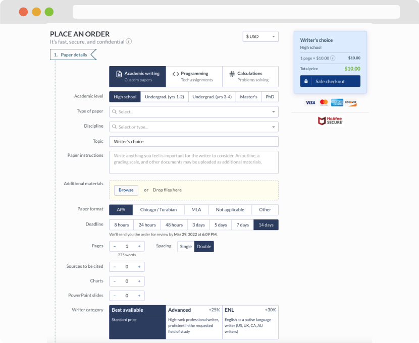
First, you will need to complete an order form. It's not difficult but, in case there is anything you find not to be clear, you may always call us so that we can guide you through it. On the order form, you will need to include some basic information concerning your order: subject, topic, number of pages, etc. We also encourage our clients to upload any relevant information or sources that will help.
Complete the order form
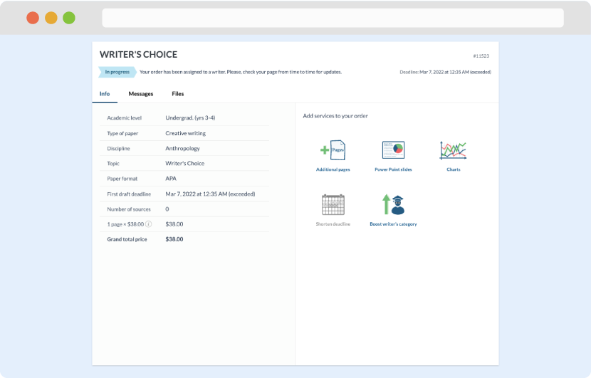
Once we have all the information and instructions that we need, we select the most suitable writer for your assignment. While everything seems to be clear, the writer, who has complete knowledge of the subject, may need clarification from you. It is at that point that you would receive a call or email from us.
Writer’s assignment
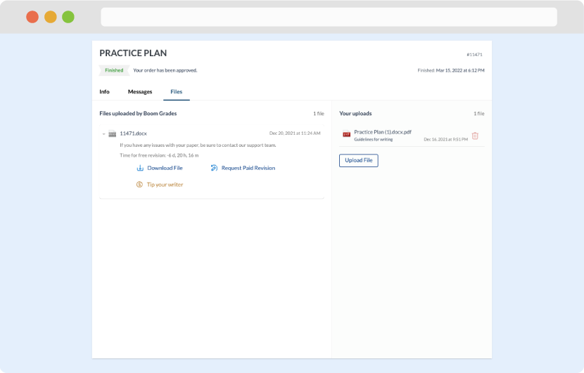
As soon as the writer has finished, it will be delivered both to the website and to your email address so that you will not miss it. If your deadline is close at hand, we will place a call to you to make sure that you receive the paper on time.
Completing the order and download