It is a fact of examination that “Tea-bag” filling procedure is the weight of the tea in the individual bags. For this brand of the tea, the labelled weight of the tea-pack refers that on an average, there are 5.5 grams of tea in a tea-bag. A small sample of “tea-packs” (50 samples) produced in an hour by a “Machine” is undertaken for analysis.
The “Mean” of the considered 50 samples is 5.5014 grams.
The “Median” of the considered samples is 5.515 grams.
The first quartile of the considered samples is 5.44 grams.
The third quartile of the considered samples is 5.57 grams.
The range of the considered samples of the tea-bags is 0.52 grams.
The “Interquartile range” (IQR) of the tea-bags are 0.13 grams.
The variance of the samples is 0.112 grams.
The “Standard deviation” (SD) of the samples is 0.10583 grams.
The “Coefficient of Variation” (CV) of the tea-bag samples is 1.924%.
The measures of central tendency indicates that average weight of the sampled tea-bags is more than 5.5 gm (Wonnacott and Wonnacott 1990). Not only that, 25% of the tea-bags and 50% of the tea-bags have weight more than 5.57 gm. and 5.515 gm. respectively. Only 25% of the tea bags have weight less than 5.44 gm. It refers that, the company is giving away their products with a significant number of tea-bags weighing more than 5.5 gm.
The measures of dispersion indicates that the difference of weights most weighted and least-weighted tea-bags is 0.52 gm. The interquartile range interprets that 75th percentile and 25th percentile tea-bags cause the weight difference of 0.13 gm. That is middle most 50% of the weighted tea-bags lies in the weight interval of 5.57 gm. and 5.44 gm. causing the difference of 0.13 gm. The standard deviation (= 0.10583 gm.) and variance (= 0.112 gm.) indicate that the scatter ness among the weights of the tea-bags is not very high. The value of coefficient of variation among the tea-bags concludes that rate of variation among the weights of tea-bags is not significantly high.
The distribution of weights of “Tea bags” depicts that the distribution is symmetric. Its median is near 5.5 gm. First quartile and minimum weight of the tea-bags is less than 5.5 gm., whereas the third quartile and maximum weight of the tea-bags is more than 5.5 gm.
The skewness of the distribution of 50 samples of the “Tea Bags” is nearly 0. The distribution is approximately normally distribution. Hence, the distribution is symmetric.
To test the claim of the tea company, whether they are packing more than 5.5 gm. tea in the bags or not, the tea company sets a hypothesis for testing.
Hypotheses:
Null hypothesis (H0): The mean weight of the sampled tea-bags is 5.5 gm.
Alternative hypothesis (H0): The mean weight of the sampled tea-bags is more than 5.5 gm.
|
One sample t-test |
|
|
Average weight |
5.5014 |
|
Hypothetical average weight |
5.5 |
|
Difference |
0.0014 |
|
Count (n) |
50 |
|
Degrees of freedom |
49 |
|
Standard deviation |
0.10583 |
|
Standard Error |
0.014967 |
|
T-statistic |
0.093541 |
|
p-value |
0.462928 |
|
Confidence interval |
95% |
|
Level of significance |
5% |
|
Sig. |
no |
The average weight of the tea-bags is 5.5014 gm., and the “Standard deviation” is 0.10583 gm. The hypothetical average weight of the “Tea-bags” is 5.5 gm. The one sample t-test is applied to test the hypothesis at 95% confidence interval. The calculated t-statistic is 0.093541 with 49 degrees of freedom. The p-value of the t-statistic is 0.462928. The calculated p-value is greater than 5%. Hence, null hypothesis could not be rejected. Also, calculated T-critical>T-statistic as 1.676>0.463. In this manner also, null hypothesis cannot be rejected (Romano and Lehmann 2005).
Therefore, it could be concluded that average weight of the 50 tea-bags is equal to 5.5 gm. with 95% probability.
Hence, the tea-company is packing 5.5 gm. of tea in the packets on an average making no losses. It could be concluded that, the proposition of the Tea Company that they are facing losses due to packaging more tea in the tea-bags is not true.
The improved process to serve customers during the noon to 1 pm is accomplished by the bank. For, examining waiting time of all the customers, the waiting time is recorded for a period of time. The waiting time of the branch of the specified bank is recorded for 15 observations.
To test the average waiting time, whether customers are waiting less than 5 minutes or not, the branch office sets a hypothesis for testing.
Null hypothesis (H0): The average weight time of the sampled people is 5 minutes.
Alternative hypothesis (H0): The average weight time of the sampled people is less than 5 minutes.
|
One sample t-test |
|
|
Average weight |
4.286667 |
|
Hypothetical average weight |
5 |
|
Difference |
0.713333 |
|
Count (n) |
15 |
|
Degrees of freedom |
14 |
|
Standard deviation |
1.637985 |
|
Standard Error |
0.422926 |
|
T-statistic |
1.686663 |
|
p-value |
0.056907 |
|
Confidence interval |
95% |
|
Level of significance |
5% |
|
Sig. |
no |
The average waiting time is 4.287 minutes and the “Standard deviation” (SD) is 0.713 minutes. The hypothetical average waiting time is 5 minutes. The one sample t-test is applied to test the hypothesis at 95% confidence interval.
When, level of significance is 5%, the calculated t-statistic is 1.68666 with 14 degrees of freedom. The p-value of the t-statistic is 0.056907. The calculated p-value is greater than 5%. Hence, null hypothesis could be accepted with 95% probability.
Therefore, it could be concluded that the average waiting time of the customers is equal to 5 minutes with 95% probability.
Hence, it could be concluded that at 5% significance level, there is not any evidence that mean waiting time is less than 5 minutes.
The first assumption is maintained that the undertaken data is continuous in nature.
The second assumption is violated as the waiting time is not approximately normally distributed.
The third assumption also violated as the box plot depicts the probable presence of outliers in the data set.
The fourth assumption is maintained as the observations are independent to each other because of these are the random samples.
If, a customer comes to branch office during lunch hour asks about the approximate waiting time; then branch manager replied about not more than 5 minutes, then manager is wrong with his/her words. Because, the analysis in segment (2.a) shows that on an average, a customer do not wait less than 5 minutes to get served. More than 5 minutes may be required to be served to any customer.
The advantage and disadvantages of using linear regression model in business:
The daily challenges of running a small business without predicting the future could be daunting. Both the Managers and operators could keep their eyes on the trend while running a company or a business. Linear regression analysis is such a type of statistical analysis technique utilised by business researchers and economists that helps the managers and business owners to forecast future situations. Linear regression model examines the association between the “Dependent” and “Independent” variables.
Linear regression analysis provides the quantitative suggestion and help to the judgment of the managers from the view-point of the fluency of the management. Hence, prediction of future is the major advantage of using linear regression model.
Business data could be large or small depending on the finance, operations and customer purchases. A proper data analysis led to make business decision (Hersey, Blanchard and Johnson 2007). It also let decision-makers to have a new insight and make policies accordingly. A manager who tries to expand his/her business in terms of sales and customer traffic in a regression may find a correlation between company revenues and facility size (Zott, Amit and Massa 2011).
Large data sets have potential to yield new information about small trades and operations (Dielman 2001). Linear regression can generate new insight for managers by uncovering relationship and pattern that was previously inherent.
Linear regression technique also can correct management considering adverse evidences (Mendenhall and Sincich 1993). It helps to find lack and mistakes of business operation to the managers.
Linear regression model is restricted to the “Straight-line Association” between response and predictors. It fails to determine the quadratic or exponential relationship among dependent variable and independent variables (Seber and Lee 2012).
Linear regression model only highlights the average of the variables. However, sometimes linear regression model focuses on the extreme values of the response variable. Average values of the variables of the regression model is actually not a description of the all values of variables (Cooper et al., 2006). Quartile regression is needed in those case.
Outliers are inevitable in actual data set. Linear regression is “Sensitive” to the outliers. Outliers may be “univariate” or “multivariate” that have vivid impact on the regression.
In case of linear regression model, data should always be independent. It is a huge restriction for constructing a linear regression model.
Correlation coefficient (R) finds the link between two factors. Coefficient of determination (R2) refers percentage of variation in dependent variable explained by “Independent variables” (Montgomery, Peck and Vining 2012). Correlation can only find the linking rate of two factors, not the association rate or explanation rate of response and predictive factors. No concept of dependent or independent factors is in the correlation coefficient. Unlike Coefficient of determination, correlation coefficient only considers “Cause” and “Effect” relation (Ozer, 1985). Hence, Coefficient of determination is better to represent the expression of association.
“A Linear regression model” is not always proper assessment for the data as the residuals and residual plots are also depict a fairly pattern (Cooper, Seiford and Zhu 2004). The residual plot verifies the linear or non-linear pattern of the “Regression Model”. A “Residual Plot” is a scatter plot that displays “Residuals” vertically and the “Predictors” horizontally. If the points of a “Residual plot” are dispersed randomly around the “Horizontal axis”, then, a “Linear Regression Model” is appropriate for the data. Otherwise, the “Non-linear model” is suitable (Zeileis and Hothorn 2002).
Reference:
Cooper, D.R., Schindler, P.S. and Sun, J., 2006. Business research methods (Vol. 9). New York: McGraw-Hill Irwin.
Cooper, W.W., Seiford, L.M. and Zhu, J., 2004. Data envelopment analysis. In Handbook on data envelopment analysis (pp. 1-39). Springer, Boston, MA.
Dielman, T.E., 2001. Applied regression analysis for business and economics. Pacific Grove, CA: Duxbury/Thomson Learning.
Hersey, P., Blanchard, K.H. and Johnson, D.E., 2007. Management of organizational behavior (Vol. 9). Upper Saddle River, NJ: Prentice hall.
Mendenhall, W. and Sincich, T., 1993. A second course in business statistics: Regression analysis. San Francisco: Dellen.
Montgomery, D.C., Peck, E.A. and Vining, G.G., 2012. Introduction to linear regression analysis (Vol. 821). John Wiley & Sons.
Ozer, D.J., 1985. Correlation and the coefficient of determination. Psychological Bulletin, 97(2), p.307.
Romano, J.P. and Lehmann, E.L., 2005. Testing statistical hypotheses.
Seber, G.A. and Lee, A.J., 2012. Linear regression analysis (Vol. 329). John Wiley & Sons.
Wonnacott, T.H. and Wonnacott, R.J., 1990. Introductory statistics (Vol. 5). New York: Wiley.
Zeileis, A. and Hothorn, T., 2002. Diagnostic checking in regression relationships.
Zott, C., Amit, R. and Massa, L., 2011. The business model: recent developments and future research. Journal of management, 37(4), pp.1019-1042.
Essay Writing Service Features
Our Experience
No matter how complex your assignment is, we can find the right professional for your specific task. Contact Essay is an essay writing company that hires only the smartest minds to help you with your projects. Our expertise allows us to provide students with high-quality academic writing, editing & proofreading services.
Free Features
Free revision policy
$10Free bibliography & reference
$8Free title page
$8Free formatting
$8How Our Essay Writing Service Works

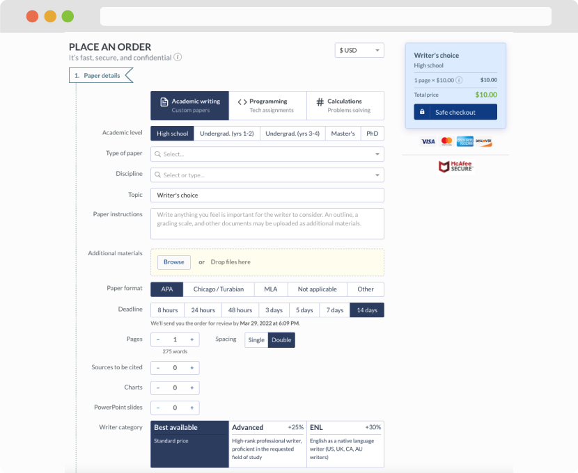
First, you will need to complete an order form. It's not difficult but, in case there is anything you find not to be clear, you may always call us so that we can guide you through it. On the order form, you will need to include some basic information concerning your order: subject, topic, number of pages, etc. We also encourage our clients to upload any relevant information or sources that will help.
Complete the order form
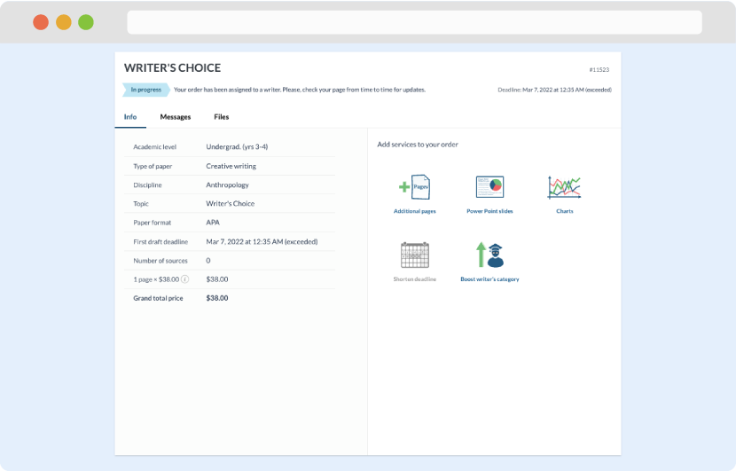
Once we have all the information and instructions that we need, we select the most suitable writer for your assignment. While everything seems to be clear, the writer, who has complete knowledge of the subject, may need clarification from you. It is at that point that you would receive a call or email from us.
Writer’s assignment
As soon as the writer has finished, it will be delivered both to the website and to your email address so that you will not miss it. If your deadline is close at hand, we will place a call to you to make sure that you receive the paper on time.
Completing the order and download