Dear Lee,
I went through the dataset and I have a made a complete analysis of the same. The answers for your questions are attached below. Hope this will provide you with the insight that you need and will help you in overcoming your problems.
Regards.
John Frank.
An overall summary of the employee working hour can be written as follows:
The required summary statistic table is :
Fig 1: Descriptive statistics
|
Column1 |
|
|
Mean |
45.26888889 |
|
Standard Error |
0.462535883 |
|
Median |
40 |
|
Mode |
40 |
|
Standard Deviation |
9.811867779 |
|
Sample Variance |
96.27274932 |
|
Kurtosis |
2.924597195 |
|
Skewness |
1.555322843 |
|
Range |
61 |
|
Minimum |
28 |
|
Maximum |
89 |
|
Sum |
20371 |
|
Count |
450 |
|
!st quartile |
40 |
|
3rd quartile |
50 |
|
IQR |
10 |
Average working time of each employee is 45.2688 hours. This average working hour can deviate in a range of 9.811 hours employees can deviate from their average working hour with 9.811 hours (Wildemuth 2016). Maximum number of employees woks for 40 hours. 50% of the employees work more than 40 hours and 50% of them works less than that. 255 of the employees work less than 40 hours and 25 % of the employees woks more than 50 hours. Median is less than mean that means distribution of working hours is left skewed which implies that the worker tends to work less regarding hours (Chang 2015). The maximum working hour for an employee is 89 hours and the minimum working hour is 28 hour. The total range of working hour is 61. The total number of employee is 450. The frequency table and box and whisker pot can be attached with the said report.
It is clear from the histrogram that there are 6 divisions of the hours of work starting from the range of 28 – 38.16667 and ending in 78.83333 – 89. The frequency distribution for each of the group is is also shown in the table.
The plot clearly shows that there is a whisker in the said frequency division.
There are 450 employees in total and number of people who are very satisfied with their job are 206 in number (Norman, Mello and Choi 2016). A frequency table for the dataset is given below:
Table 2: Frequency distribution of the dataset.
|
Row Labels |
Count of Moderately satisfied |
|
A little dissatisfied |
29 |
|
Moderately satisfied |
194 |
|
Very dissatisfied |
20 |
|
Very satisfied |
206 |
|
Grand Total |
449 |
A bar chart showing the frequency distribution of the whole dataset will be like:
Therefore. Assuming p to be the proportion of people who are most likely to retain their job, then:
p = 0.547.
So, 1 – p = 0.542.
Therefore. Standard deviation of proportion is 0.023 and standard error is 0.046.
Hence, the upper and lower limit of this proportion are (0.41, 0.50).
It can be said here that people who are likely to retain their job are 0.046 in proportion and this proportion can vary with a highest limit of 0.50 and in the lowest limit of 0.41.
Y = a + b*x where y is the dependent variable and x is the independent variable. a and b are regression constants. The calculated table is:
Fig 2: Regression calculation.
|
SUMMARY OUTPUT |
||||||||
|
Regression Statistics |
||||||||
|
Multiple R |
0.303019 |
|||||||
|
R Square |
0.091821 |
|||||||
|
Adjusted R Square |
0.089794 |
|||||||
|
Standard Error |
0.471741 |
|||||||
|
Observations |
450 |
|||||||
|
ANOVA |
||||||||
|
df |
SS |
MS |
F |
Significance F |
||||
|
Regression |
1 |
10.07987 |
10.07987 |
45.29467 |
5.2E-11 |
|||
|
Residual |
448 |
99.6979 |
0.22254 |
|||||
|
Total |
449 |
109.7778 |
||||||
|
Coefficients |
Standard Error |
t Stat |
P-value |
Lower 95% |
Upper 95% |
Lower 95.0% |
Upper 95.0% |
|
|
Intercept |
1.1135 |
0.105094 |
10.59532 |
1.47E-23 |
0.906962 |
1.320038 |
0.906962 |
1.320038 |
|
X Variable 1 |
-0.01527 |
0.002269 |
-6.73013 |
5.2E-11 |
-0.01973 |
-0.01081 |
-0.01973 |
-0.01081 |
It can be said from calculation that intercept or a is 1.113 and p value for this is 1.47E-23 which is less than 0.05 (Colchero et al. 2016.). Therefore, the intercept value can be accepted. Again, X-variable value or b is -0.015 with p-value 5.2E-11 which is again less than 0.05. Therefore, X-variable value can again be accepted. F-statistic for the regression analysis is 45.29 and F-significant value is 5.2E-11 which is less than f statistic value (Ladd et al. 2014.). Therefore, the regression fit is statistically significant. The R-square value is 0.09 which means that the estimates can differ within a range of 0.09.The regression line can be interpreted as:
Y = 0.003 + (-0.015)*x.
Worker influence levels can be classified into 4 levels like influences always, influences at times, influences much of the times, and never influences (Solon, Haider and Wooldridge 2015). Again, there are 152 people who always influences, 66 people who influences much of the times, 181 peoples who influences much of the times and 51 people who never influences. The frequency distribution of the whole dataset will be like:
Table 3: Frequncy distribution of influence of the workers.
|
Row Labels |
Count of Sometimes |
|
Always |
152 |
|
Much of the time |
181 |
|
Never |
51 |
|
Sometimes |
65 |
|
Grand Total |
449 |
A bar chart depicting the frequency distribution here will be like:
Figure 4: Frequnecy distribution of influence.
Therefore, it can be said that most of the workers influences company decisions. Mostly of them do that always. There are only a very low number of workers who doesn’t have any influence at all (Plesinger et al. 2015).
Work hours can be related to education years, salary, work years and years of experience in Cuteen. The relation equation or the regression equation can be written as:
y = a + b*x1 + cx2 + d*x3,
where, y is the dependent variable, x is the independent variable, a is the intercept of regression and b, c and d are the regression co efficient.
The required calculated table is:
Fig 3: Regression table.
|
Regression Statistics |
Column1 |
|
Multiple R |
0.190687108 |
|
R Square |
0.036361573 |
|
Adjusted R Square |
0.0298797 |
|
Standard Error |
9.664168273 |
|
Observations |
450 |
|
ANOVA |
Column1 |
Column2 |
Column3 |
Column4 |
Column5 |
|
df |
SS |
MS |
F |
Significance F |
|
|
Regression |
3 |
1571.782253 |
523.927418 |
5.60973259 |
0.000879492 |
|
Residual |
446 |
41654.68219 |
93.3961484 |
||
|
Total |
449 |
43226.46444 |
|
Column1 |
Coefficients |
Standard Error |
t Stat |
P-value |
Lower 95% |
Upper 95% |
Lower 95.0% |
Upper 95.0% |
|
Intercept |
42.25530642 |
1.249459475 |
33.8188691 |
3.594E-125 |
39.79974731 |
44.71086552 |
39.79974731 |
44.71086552 |
|
X Variable 1 |
0.138186906 |
0.033857344 |
4.08144551 |
5.3036E-05 |
0.071647165 |
0.204726648 |
0.071647165 |
0.204726648 |
|
X Variable 2 |
-0.035420588 |
0.056579799 |
-0.6260289 |
0.53161625 |
-0.146616704 |
0.075775529 |
-0.146616704 |
0.075775529 |
|
X Variable 3 |
-0.041514931 |
0.066593935 |
-0.6234041 |
0.53333768 |
-0.172391799 |
0.089361937 |
-0.172391799 |
0.089361937 |
It can be said from the calculation that intercept or a is 42.25530642 and the corresponding p value is3.594E-125 which is less than 0.05 and that means the intercept value can be accepted (Boos and Osborne 2015.). Again, b or coefficient of x1 is 0.138186906 and the corresponding p – value is 5.3036E-05 which is less than 0.05 that is the value will be accepted. C or co-efficient of x2 is 0.035420588 and the corresponding p-value is 0.53161625 which is less than 0.05 and therefore, the value can be accepted. D or coefficient of x3 is 0.041514931 and the corresponding p-value is 0.53333768 which is more than 0.05. therefore, the intercept value cannot be accepted. Again, regressed F-statistic value is 7.899 and the significant f_value is 3.82E-05 which is less than f statistic value and therefore, the regression value can be accepted here (Thiem 2014). The R-square value is 0.05 that means the fitted value can deteriorate within a range of 0.05. The fitted regression line is :
Y = 42.25 + (0.1381)*x1 + (0.0354)*x2 .
A scatter plot can be shown among the dependent and the independent variables.
Scatter plot between working hours and salary.
References:
Solon, G., Haider, S.J. and Wooldridge, J.M., 2015. What are we weighting for?. Journal of Human resources, 50(2), pp.301-316.
Boos, D.D. and Osborne, J.A., 2015. Assessing variability of complex descriptive statistics in monte carlo studies using resampling methods. International Statistical Review, 83(2), pp.228-238.
Campbell, F., Conti, G., Heckman, J.J., Moon, S.H., Pinto, R., Pungello, E. and Pan, Y., 2014. Early childhood investments substantially boost adult health. Science, 343(6178), pp.1478-1485.
Chang, K.T., 2015. Introduction to geographic information systems. McGraw-Hill Science/Engineering/Math.
Colchero, M.A., Popkin, B.M., Rivera, J.A. and Ng, S.W., 2016. Beverage purchases from stores in Mexico under the excise tax on sugar sweetened beverages: observational study. bmj, 352, p.h6704.
Kuppuswamy, V. and Bayus, B.L., 2018. Crowdfunding creative ideas: The dynamics of project backers. In The Economics of Crowdfunding (pp. 151-182). Palgrave Macmillan, Cham.
Ladd, J., Hsieh, Y.H., Barnes, M., Quinn, N., Jett-Goheen, M. and Gaydos, C.A., 2014. Female users of internet-based screening for rectal STIs: descriptive statistics and correlates of positivity. Sex Transm Infect, 90(6), pp.485-490.
Norman, C., Mello, M. and Choi, B., 2016. Identifying frequent users of an urban emergency medical service using descriptive statistics and regression analyses. Western Journal of Emergency Medicine, 17(1), p.39.
Phoa, F.K.H., Chou, S.K. and Woods, D.C., 2017. Summary of effect aliasing structure (SEAS): new descriptive statistics for factorial and supersaturated designs. arXiv preprint arXiv:1711.11488.
Plesinger, F., Klimes, P., Halamek, J. and Jurak, P., 2015, September. False alarms in intensive care unit monitors: detection of life-threatening arrhythmias using elementary algebra, descriptive statistics and fuzzy logic. In Computing in Cardiology Conference (CinC), 2015 (pp. 281-284). IEEE.
Thiem, A., 2014. Membership function sensitivity of descriptive statistics in fuzzy-set relations. International Journal of Social Research Methodology, 17(6), pp.625-642.
Utinans, A., Ancane, G., Tobacyk, J.J., Boyraz, G., Livingston, M.M. and Tobacyk, J.S., 2015. Paranormal beliefs of latvian college students: a latvian version of the revised paranormal belief scale. Psychological reports, 116(1), pp.116-126.
Wildemuth, B.M. ed., 2016. Applications of social research methods to questions in information and library science. ABC-CLIO.
Essay Writing Service Features
Our Experience
No matter how complex your assignment is, we can find the right professional for your specific task. Contact Essay is an essay writing company that hires only the smartest minds to help you with your projects. Our expertise allows us to provide students with high-quality academic writing, editing & proofreading services.
Free Features
Free revision policy
$10Free bibliography & reference
$8Free title page
$8Free formatting
$8How Our Essay Writing Service Works

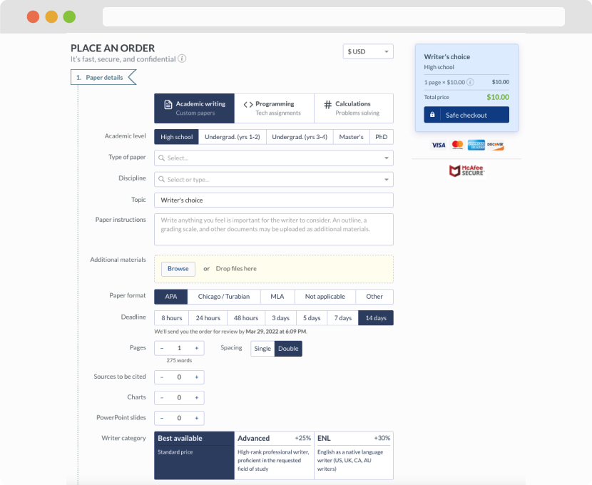
First, you will need to complete an order form. It's not difficult but, in case there is anything you find not to be clear, you may always call us so that we can guide you through it. On the order form, you will need to include some basic information concerning your order: subject, topic, number of pages, etc. We also encourage our clients to upload any relevant information or sources that will help.
Complete the order form
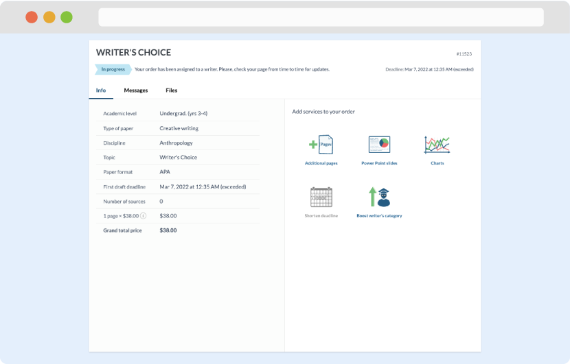
Once we have all the information and instructions that we need, we select the most suitable writer for your assignment. While everything seems to be clear, the writer, who has complete knowledge of the subject, may need clarification from you. It is at that point that you would receive a call or email from us.
Writer’s assignment
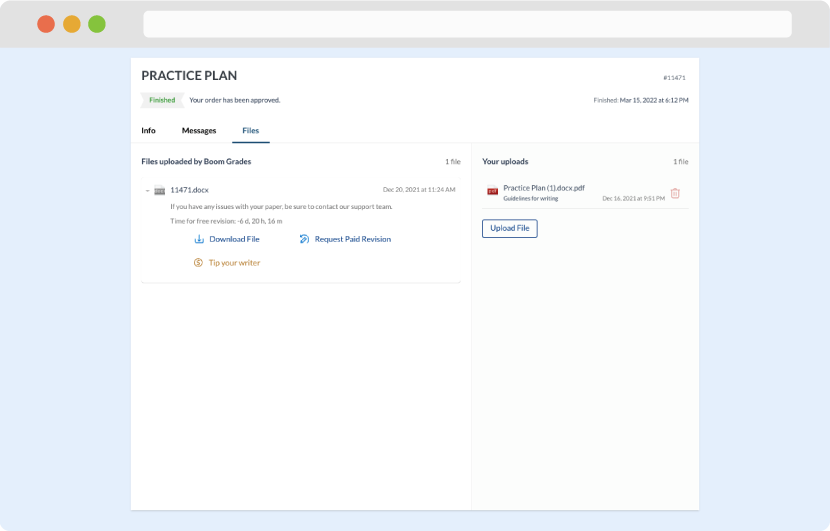
As soon as the writer has finished, it will be delivered both to the website and to your email address so that you will not miss it. If your deadline is close at hand, we will place a call to you to make sure that you receive the paper on time.
Completing the order and download