Transport survey data are collected worldwide to aid in modelling and planning of the transport system in any particular country (Zmud et al., 2013). Various methods of survey and data collection are utilized to ensure the data collected for interpretation is reliable and of high quality (Fairnie, Wilby and Saunders, 2016). This method ranges from face to face interviews to more advanced methods that involve the use of modern technologies such as mobile phones and computer applications. However, Shen et.al. (2016) argues that during the process of data collection and interpretation there are always biases that result from survey methods and poor handling of data leading to the data obtained not providing the accurate expected results to aid in planning, modelling and improvement of the transport system.
The purpose of this paper is therefore, to test the skills of collection of both primary and secondary data, interpreting the data and providing the correct numeric summaries, display appropriate graphs and utilize statistical inference to assist the NSW government in making conclusive and reliable recommendations on how to improve public transport.
Dataset 1 is data that has been obtained from the Transport for NSW Open Data website(Opendata.transport.nsw.gov.au, 2016). It has been edited to include only a few cases and variables to be used in answering specific transport related research questions (. On the basis of being “Second hand”, i.e. not collected by the researcher, it can be described as secondary data (Ullah, 2014). The data set has six variables namely mode, date, tap, time, loc and count. Mode is a categorical variable that indicates the type of the public transport, date is a quantitative continuous variable that indicates date of the tap on/off held, tap is a categorical variable indicating whether tap is on or off, loc is a categorical variable indicating locations of stops which in the case of buses are postal codes and for other modes of transport are names of locations. Lastly, count is numeric variable indicating the total number of tap on or off on certain location and date (Donges, 2018). The mode variable has four cases namely Bus, Train, Ferry and Light Rail, tap has two cases on and off and loc has two cases namely postal code and station name (Lock et al., 2013).
Dataset 2 is collected from first hand survey to show the preference of different genders for the various modes of transport. It is collected by directly interviewing individuals for their preferred mode of transport (Fowler, 2009). Due to the fact that its collected by the researcher directly interviewing the respondent it can be described as primary data (Ullah, 2014). A total of 81 individuals comprising both male and female are surveyed. This large sample is preferred for better accuracy. It has three variables; Date which indicates the date when the survey was taken, gender is a categorical variable indicating whether a person is male or female and finally mode is a categorical variable indicating the preferred mode of transport (Donges, 2018). Like in dataset 1, mode has Bus, Train, Ferry and Light Rail as the cases while gender has male and female (Lock et al., 2013). The limitation of this this data set it is concentrated for a specific group of individuals in a particular region, therefore the overall trend of the data does not follow that the NSW secondary data that is collected for vast group of individuals from different locations resulting to some level of inaccuracy (DeFranzo, 2014).
Section 2
Analysis of Single Variable in Dataset 1
To determine the mode of transport that is most used by the NSW people during 8th-14th of August we use proportion of the total and the count of total.
From the table of summary statistics above, the count indicates that most people used bus, followed by train, then ferry and lastly light trail. The same is depicted by the proportion column; buses have the highest proportion of preference, followed by train, ferry and lastly light trail.
To visualize the most commonly used mode of transport, a pie chart or a bar chart can be used. The pie chart visualizes proportion as percentage of the total thereby the mode with greatest preference occupies the greatest percentage in the pie chart (Wesley, 2018).
From the pie chart above, the proportions as percentage of the total for the various modes of transport are displayed.
The bar chart represents the most commonly used mode of transport as a sum of count (Wesley, 2018). The most commonly used mode of transport has the highest count while the least commonly used mode of transport has the lowest count.
From all the cases above; statistical summary, pie chart and bar chart buses were the most commonly used mode of transport by NSW people, followed by train, the ferry and finally the ferry.
We carry out a hypothesis test to examine whether there are more that 50% of public transport users in NSW use buses as the particular mode of transport by setting up an appropriate hypothesis, perform the test.
The proportion of people using buses is 0.48, hence our Phat=0.48 our sample size N =1000. We state the null and alternate hypothesis:
Checking whether the assumptions are something to go by:
From the above, all the assumptions are satisfied hence we can proceed to determine the values of P for normal distribution. The test statistic for proportion will be given by;
The default level of significance is taken as 0.05. For this level of significance, the decision rule will be reject Ho if Z is to the left of -1.96 or if Z is to the right of 1.96 or of P value is less than the significance level (Schenkelberg, 2017). In our case the Z value (-1.26) is to the right of -1.96 and P(Z>-1.26) =0.104 is greater than the significance level, we cannot reject the null hypothesis and therefore it would be okay to conclude that more than 50% of the NSW people use buses as their preferred mode of transport.
Section 3
Analysis of Two Variable Dataset 1
We need to prepare a recommendation for whether the NSW government should go ahead with its plan to build an underground Railway line from either Parramatta, Banks town, or Gosford to central.
The summary statistics for the above railways stations is as shown below:
From the above summary statistics, Parramatta station has a mean of 466.667, followed by Banks town with a mean of 104.400 and Lastly Gosford Station with a mean of 47.667. the minimum and maximum for Banks town is 23 and 190 respectively, for Parramatta station its 91 and 1425 respectively and for the Gosford station its 34 and 63. By just observing the summary statistics above NSW government should consider building the underground railway at the Parramatta station to central to minimize congestion and the high numbers that are served by the station.
To visualize the above data, we use the box plot shown below. The Box plot will interpret the data in terms of quartiles and skewness (Krzywinski and Altman, 2014). From the box plot the Parramatta box plot is skewed to the right with a maximum of 1425. Its followed by the Banks town station which is somehow not skewed in either left or right. From the boxplots again, it under railway can be recommended to be built in the Parramatta station to central.
Our null hypothesis H0: All means are equal and the alternate hypothesis Hi: There is a difference in means.
We proceed to use “ANOVA for difference in means” in Stat Key. we load the data click ANOVA Table and record the important
From the above, we can check whether the assumptions are anything to go by. The sample size (n) in each of the cases is greater than 30 and the no standard deviation in either case is greater than twice the other hence all the assumptions are satisfied. The ANOVA table helps us determine the numerator degrees of freedom and the denominator degrees of freedom to be used in determination of the p value for F distribution (Rumsey, 2007). The numerator degree of freedom is one while the denominator degrees of freedom is 998.
The p value is determined as below in Stat Key software using the graph of F distribution(Lock5stat.com, 2018).
The P value determined is 0.025. Since the P value obtained is less than the significance level of 0.05 we reject the null hypothesis and conclude that there is sufficient evidence for the difference in mean
Section 4
Collection and Analysis of Dataset 2
The data is collected by surveying a group of individuals comprising of male and female and their preferred mode of transport.
The whole sample comprises of 81 individuals. It is made large enough to increases the accuracy of the results obtained (Nayak, 2010). The summary statics showing the various genders
The above statistical summary show that a total of 50 female individuals and 31 male individuals were surveyed. Of the 50 female 22 prefer light rail, 7 prefer ferry, 16 prefer bus and 5 prefer train. On the other hand, 5 male prefer light rail, 7 ferry, 16 bus, and 3 train. Buses are the most preferred mode of transport with 32 individuals, followed by light rail, then ferry and finally train. The above statistical summary can be summarized using a stacked bar chart
Section 5
Discussion and Conclusion
The above data interpretations show that the most commonly used mode of transport is buses with over 50% of the population proportion. It is followed by train, ferry and light rail tails the list. In terms of gender, more females prefer using light rails while more mail prefer buses. Therefore, we can recommend to the NSW government to consider improving the road transport network since it’s the most commonly used mode of transport. However, due to preference choices varying from individual to individual, it should not down its tools in improving other modes of transport. On the hand, the construction of the underground rail to central should be done at Parramatta station becomes it offers more service compared to the rest of the stations. This would ease congestion in this station as well as increase efficiency and effectiveness of the station. For the purpose of the future development to enhancement of the transport system, the NSW government should conduct research on the quality of service offered by the transport entities to know how they influence their choice of a transport system, so that it can know how to adjust to meet customers demand for all the sectors.
References
DeFranzo, S. (2014). Advantages and disadvantages of face-to-face data collection. [online] Snap Surveys. Available at: https://www.snapsurveys.com/blog/advantages-disadvantages-facetoface-data-collection/ [Accessed 17 Sep. 2018].
Donges, N. (2018). Data types in statistics – towards data science. [online] Towards DataScience. Available at: https://towardsdatascience.com/data-types-in-statistics-347e152e8bee [Accessed 17 Sep. 2018].
Fairnie, G., Wilby, D. and Saunders, L. (2016). Active travel in London: The role of travel survey data in describing population physical activity. Journal of Transport & Health,3(2).
Fowler, F. (2009). Survey research methods. 4th ed. London: Sage Publication.
Lock, R., Lock, P., Morgan, K., Lock, E. and Lock, D. (2013). Statistics: Unlocking the power of data. 1st ed. Hoboken, N.J.: Wiley.
Lock5stat.com. (2018). Theoretical distribution. [online] Available at: https://www.lock5stat.com/StatKey/theoretical_distribution/theoretical_distribution.html#normal [Accessed 17 Sep. 2018].
Krzywinski, M. and Altman, N. (2014). Points of Significance: Visualizing samples with boxplots. [online] Nature Methods. Available at: https://www.nature.com/articles/nmeth.2813 [Accessed 17 Sep. 2018].
Nayak, B. (2010). Understanding the relevance of sample size calculation. [online] NCBI. Available at: https://www.ncbi.nlm.nih.gov/pmc/articles/PMC2993974/ [Accessed 17 Sep. 2018].
Opendata.transport.nsw.gov.au. (2016). Opal Tap On and Tap Off | TfNSW Open Data Hub and Developer Portal. [online] Available at: https://opendata.transport.nsw.gov.au/dataset/opal-tap-on-and-tap-off [Accessed 17 Sep. 2018].
Rumsey, D. (2007). Intermediate statistics for dummies. 1st ed. Hoboken, N.J.: Wiley.
Schenkelberg, F. (2017). Hypothesis tests for Proportion – Accendo Reliability. [online] Accendo Reliability. Available at: https://accendoreliability.com/hypothesis-tests-for-proportion/ [Accessed 17 Sep. 2018].
Shen, L. et al., 2016. The future direction of household travel surveys methods in Australia. Australian transport forum incorporated. Available at: https://atrf.info/papers/2016/files/ATRF2016_Full_papers_resubmission_115.pdf [Accessed September 17, 2018].
Ullah, M. (2014). Primary and secondary data in statistics. [online] Basic Statistics and Data Analysis. Available at: https://itfeature.com/statistics/primary-and-secondary-data-in-statistics [Accessed 17 Sep. 2018].
Wesley, S. (2018). Top 5 best data visualization techniques for 2018. [online] Big Data Made Simple – One source. Many perspectives. Available at: https://bigdata-madesimple.com/top-5-best-data-visualization-techniques-for-2018/ [Accessed 17 Sep. 2018].
Zmud, J., Lee-Gosselin, M., Munizaga, M. and Carrasco, J. (2013). Transport survey methods. Bingley: Emerald Group Publishing Limited.
Essay Writing Service Features
Our Experience
No matter how complex your assignment is, we can find the right professional for your specific task. Contact Essay is an essay writing company that hires only the smartest minds to help you with your projects. Our expertise allows us to provide students with high-quality academic writing, editing & proofreading services.
Free Features
Free revision policy
$10Free bibliography & reference
$8Free title page
$8Free formatting
$8How Our Essay Writing Service Works

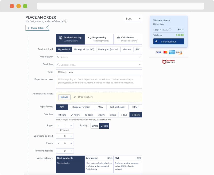
First, you will need to complete an order form. It's not difficult but, in case there is anything you find not to be clear, you may always call us so that we can guide you through it. On the order form, you will need to include some basic information concerning your order: subject, topic, number of pages, etc. We also encourage our clients to upload any relevant information or sources that will help.
Complete the order form
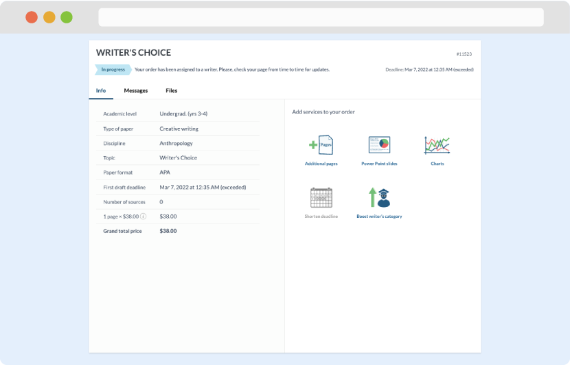
Once we have all the information and instructions that we need, we select the most suitable writer for your assignment. While everything seems to be clear, the writer, who has complete knowledge of the subject, may need clarification from you. It is at that point that you would receive a call or email from us.
Writer’s assignment
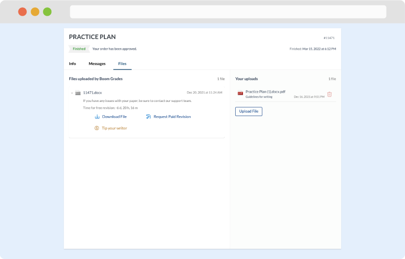
As soon as the writer has finished, it will be delivered both to the website and to your email address so that you will not miss it. If your deadline is close at hand, we will place a call to you to make sure that you receive the paper on time.
Completing the order and download