This study sought to apply statistical knowledge learnt in class in analyzing real data. I obtained my dataset from the internet, the link to the dataset is given The data contains 60 observations with a total of four variables (two categorical and two numerical/quantitative variables) namely
|
Variable |
Type |
|
Prior Sexual Experience |
Categorical |
|
Dose of Drug |
Categorical |
|
Numerical/Quantitative |
|
|
Age of the respondent |
Numerical/Quantitative |
Analysis of One Quantitative Variable
The first analysis done is looking at the summary statistics of one of the quantitative variable. Some of the measures analyzed include, mean, median, minimum, maximum, mode, standard deviation, skewness and kurtosis of the data.
|
Table 1: Descriptive statistics (Quantitative data): |
|
|
Statistic |
Sexual Activity Index |
|
Nbr. of observations |
60 |
|
Minimum |
9.370 |
|
Maximum |
23.550 |
|
Range |
14.180 |
|
1st Quartile |
12.405 |
|
Median |
15.020 |
|
3rd Quartile |
17.323 |
|
Mean |
15.152 |
|
Variance (n-1) |
9.593 |
|
Standard deviation (n-1) |
3.097 |
|
Variation coefficient |
0.203 |
|
Skewness (Pearson) |
0.297 |
|
Kurtosis (Pearson) |
-0.547 |
|
Lower bound on mean (95%) |
14.352 |
|
Upper bound on mean (95%) |
15.952 |
As we can see from the table, the average sexual activity index of the respondents is 15.152 with a median of 15.02. The maximum and minimum sexual activity index are 9.37 and 23.55 respectively. The 95% confidence interval for the sample mean showed that the range is between 14.352 (lower bound on the mean) and 15.952 (upper bound on the mean).
Also measured were the Skewness and Kurtosis; skewness measures the distribution symmetry of the dataset. The skewness and kurtosis values are close to zero implying that the data could have come from a normally distributed dataset.
Table 2 below gives the normality test. Both the Kolmogorov-Smirnov test and Shapiro-Wil test showed were insignificant (p-value > 0.05). We thus fail to reject the null hypothesis and conclude that the data is normally distributed at % level of significance.
|
Table 2: Tests of Normality |
||||||
|
Kolmogorov-Smirnova |
Shapiro-Wilk |
|||||
|
Statistic |
df |
Sig. |
Statistic |
df |
Sig. |
|
|
Sexual Activity Index |
.094 |
60 |
.200* |
.974 |
60 |
.226 |
|
*. This is a lower bound of the true significance. |
||||||
|
a. Lilliefors Significance Correction |
Next a histogram of the sexual activity index is presented and as can be seen the data seems to be normally distributed though not perfect as is expected of the bell-shaped curve.The above boxplot shows that there is no any outlier in the dataset and that the data seems to be normally distributed.
Analysis of One Categorical Variable
In analyzing one categorical variable the study considered analyzing dose of drug taken by the respondents. There were three dosage namely vehicle, 10 mg ad 15 mg. Table 3 below presents the frequency table for the categorical variable dose of drug. As can be seen in the table, equal number of respondents took the three different dosage, i.e. 33.3% (n = 20) took vehicle, another 33.3% (n = 20) took 10 mg and the remaining 33.3% (n = 20) took 15 mg.
|
Table 3: Dose of Drug |
|||||
|
Frequency |
Percent |
Valid Percent |
Cumulative Percent |
||
|
Valid |
Vehicle |
20 |
33.3 |
33.3 |
33.3 |
|
10 mg |
20 |
33.3 |
33.3 |
66.7 |
|
|
15 mg |
20 |
33.3 |
33.3 |
100.0 |
|
|
Total |
60 |
100.0 |
100.0 |
The above can also be visualized in the bar chart presented below;
Analysis of One Relationship between Two Categorical Variables:
In analyzing relationship between two categorical variable, the study considered Prior Sexual Experience and Dose of Drug.
The following hypothesis was tested using Chi-Square test of association;
H0: There is no association between Prior Sexual Experience and Dose of Drug.
H1: There is association between Prior Sexual Experience and Dose of Drug.
This was tested at 5% level of significance.
To test the above hypothesis, a Pearson Chi-Squared (χ2) test of independence (association) was used.
|
Table 4: Dose of Drug * Prior Sexual Experience: Cross tabulation |
|||||
|
Prior Sexual Experience: |
Total |
||||
|
No Sexual Experience |
Prior Sexual Experience |
||||
|
Dose of Drug |
Vehicle |
Count |
10 |
10 |
20 |
|
Expected Count |
10.0 |
10.0 |
20.0 |
||
|
10 mg |
Count |
10 |
10 |
20 |
|
|
Expected Count |
10.0 |
10.0 |
20.0 |
||
|
15 mg |
Count |
10 |
10 |
20 |
|
|
Expected Count |
10.0 |
10.0 |
20.0 |
||
|
Total |
Count |
30 |
30 |
60 |
|
|
Expected Count |
30.0 |
30.0 |
60.0 |
As can be seen in the above table (table 4), there is no any difference in terms of prior sexual experience of respondents and the dose of drug. The count and expected counts are equal across all the columns and rows.
|
Chi-Square Tests |
|||
|
Value |
df |
Asymp. Sig. (2-sided) |
|
|
Pearson Chi-Square |
.000a |
2 |
1.000 |
|
Likelihood Ratio |
.000 |
2 |
1.000 |
|
Linear-by-Linear Association |
.000 |
1 |
1.000 |
|
N of Valid Cases |
60 |
||
|
a. 0 cells (0.0%) have expected count less than 5. The minimum expected count is 10.00. |
A chi-square test of association was performed to determine whether there was association between prior sexual experience of respondents and the dose of drug taken by the respondents. There was no association between prior sexual experience of respondents and the dose of drug taken by the respondents, = 0.000, p > .05. We can conclude that prior sexual experience of the respondent does not significantly influence the dose of drug taken by the respondent.
Analysis of One Relationship between a Categorical Variable and a Quantitative Variable
This section sought to analyze One Relationship between a Categorical Variable and a Quantitative Variable. The relationship we looked at is that between prior sexual experience and sexual activity index. The hypothesis we sought to test is;
H0: The mean sexual activity index for the respondents with prior sexual experience is the same as that of the respondents with no prior sexual experience
H1: The mean sexual activity index for the respondents with prior sexual experience is different from that of the respondents with no prior sexual experience.
This was tested at 5% level of significance.
In testing the hypothesis, an independent t-test was used. This test is usual when comparing the two groups of data sets like in our case.
|
Table 6: Group Statistics |
|||||
|
Prior Sexual Experience: |
N |
Mean |
Std. Deviation |
Std. Error Mean |
|
|
Sexual Activity Index |
No Sexual Experience |
30 |
13.8967 |
2.66063 |
.48576 |
|
Prior Sexual Experience |
30 |
16.4067 |
3.02956 |
.55312 |
Table 6 above gives the group statistics. As can be seen, the average sexual activity index for the respondents with prior sexual experience is 16.41 while that of the respondents with no sexual experience is 13.90. Respondents with prior sexual experience have a much higher sexual activity index when compared to the respondents with no prior sexual experience.
|
Table 7: Independent Samples Test |
||||||||||
|
Levene’s Test for Equality of Variances |
t-test for Equality of Means |
|||||||||
|
F |
Sig. |
t |
df |
Sig. (2-tailed) |
Mean Difference |
Std. Error Difference |
95% Confidence Interval of the Difference |
|||
|
Lower |
Upper |
|||||||||
|
Sexual Activity Index |
Equal variances assumed |
.194 |
.661 |
-3.410 |
58 |
.001 |
-2.51 |
.73614 |
-3.98 |
-1.036 |
|
Equal variances not assumed |
-3.410 |
57.05 |
.001 |
-2.51 |
.73614 |
-3.98 |
-1.036 |
An independent samples t-test was conducted so as to be able to make a comparison in the mean sexual activity index for the respondents with prior sexual experience and that of the respondents with no prior sexual experience. There was a significant difference in the sexual activity index for the respondents with prior sexual experience (M = 16.41, SD = 3.03) and respondents with no prior sexual experience (M = 13.90, SD = 2.66) conditions; t (58) = -3.41, p = 0.001 (< 0.05). These results suggest that prior sexual experience really does have an effect on the sexual activity index. Specifically, our results suggest that respondents with prior sexual experience have higher sexual activity index compared to the respondents with no prior sexual experience.
The boxplots above further attempts to visualize the differences in the sexual activity index based on the prior sexual experience. As can be seen, the mean sexual activity index for those with prior sexual experience is much higher compared to that of the respondents with no prior sexual experience. No outliers were observed in any of the two box plots.
Analysis of One Relationship between Two Quantitative Variables
This section sought to analyze the relationship that exists between two quantitative variables. We considered age of the respondent and the sexual activity index. Pearson correlation test was done to check on the relationship that exists between the two variables based on the coefficient that exists.
|
Table 8: Correlations |
|||
|
Sexual Activity Index |
Age of the respondents |
||
|
Sexual Activity Index |
Pearson Correlation |
1 |
-.460** |
|
N |
60 |
60 |
|
|
Age of the respondents |
Pearson Correlation |
-.460** |
1 |
|
Sig. (2-tailed) |
.000 |
||
|
N |
60 |
60 |
|
|
**. Correlation is significant at the 0.01 level (2-tailed). |
As can be seen n table 8 above, the Pearson correlation coefficient is -0.460 and the relationship is significant at 5% level of significance (r = -0.460, p < 0.05). The negative coefficient means that there is a negative relationship between the two variables (sexual activity index and age of the respondents). Negative linear relationship means that an increase in the age of the respondent would result to a decrease in the sexual activity of the respondent while a decrease in the age would result to an increase in the sexual activity index.
A negative linear relationship can be observed between the two variables.
Regression model
To further understand how age of the respondent affects the sexual activity index, a regression equation model was constructed.The linear equation model is Where is the constant coefficient while is the coefficient for the independent variable “respondent’s age”.
The model summary table (table 9) presents the value of R, R-Square, adjusted R-Square and the standard error of the estimate. The value of R-Squared is 0.211, this basically means that 21.1% of the variation in the sexual activity index (dependent variable) is explained by the independent variable (age of the respondent). This value is quite small, implying that the larger proportion is explained by other variables outside the model.
|
Table 9: Model Summary |
||||
|
Model |
R |
R Square |
Adjusted R Square |
Std. Error of the Estimate |
|
1 |
.460a |
.211 |
.198 |
2.77418 |
|
a. Predictors: (Constant), Age |
The regression model was found to be fit and appropriate in predicting the sexual activity index using the explanatory variable “Age of the respondent” (p < 0.05). see table 10 below.
|
Table 10: ANOVAa |
|||
|
Model |
Sum of Squares |
df |
|
|
1 |
Regression |
119.587 |
1 |
|
Residual |
446.373 |
58 |
|
|
Total |
565.960 |
59 |
|
|
a. Dependent Variable: Sexual Activity Index |
|||
|
b. Predictors: (Constant), Age |
Looking at table 11 presented below, we observe that the coefficient of the intercept (constant) is 18.336; this implies that when all other factors are held constant we would expect the sexual activity index to be 18.336. Lastly, the coefficient of the explanatory variable (Age of the respondent) is -0.082; this implies that a unit increase in the age of the respondent would result to a decrease in the sexual activity index of the respondent. Similarly, a unit decrease in the age of the respondent would result to an increase in the sexual activity index of the respondent by 0.082. It is important to note that the respondent was found to be significant in the model (p < 0.05).
|
Table 11: Coefficientsa |
||||||
|
Model |
Unstandardized Coefficients |
Standardized Coefficients |
t |
Sig. |
||
|
B |
Std. Error |
Beta |
||||
|
1 |
Age of the respondent |
-.082 |
.021 |
-.460 |
-3.942 |
.000 |
|
a. Dependent Variable: Sexual Activity Index |
Conclusion
This study utilized data on prior sexual experience and dose of an androgen. The idea was to present statistical analysis of the dataset. Summary statistics was done to identify the nature of the dataset where it was found that the data comes from a normally distributed dataset with a mean computed to be 15.152.
The maximum and minimum sexual activity index was found to be 9.37 and 23.55 respectively while the 95% confidence interval for the sample mean showed that the range is between 14.352 (lower bound on the mean) and 15.952 (upper bound on the mean). No outliers were observed. In terms relationships, we observed that age is one of the crucial factors that influence the sexual activity behavior. Prior sexual experience was also identified as a factor that influences the sexual activity index. There is however no association between Prior Sexual Experience and Dose of Drug; Chi-Square test was found to be insignificant at 5% level of significance.
References
Cook, L., & Fleming, C. (2007). Analysis of clinic attendances by under-14s to sexual health clinics in Gwent. Journal of Family Planning and Reproductive Health Care, 33(1), 23-26.
Hubert, M., & Vandervieren , E. (2008). An adjusted boxplot for skewed distributions . Computational Statistics and Data Analysis, 52(12), 5186–5201.
John , A. R. (2006). Mathematical Statistics and Data Analysis.
Plackett, R. L. (2003). Karl Pearson and the Chi-Squared Test. International Statistical Review. International Statistical Institute (ISI), 51(1), 59–72.
Smith, A. (2009). Young people’s contraception and sexual health: Report of a local needs assessment in Staveley. Journal of Family Planning and Reproductive Health Care, 27(1), 29.
Waegeman, W., & De , B. B. (2008). ROC analysis in ordinal regression learning: Pattern Recognition Letters. 29, 1–9.
Essay Writing Service Features
Our Experience
No matter how complex your assignment is, we can find the right professional for your specific task. Contact Essay is an essay writing company that hires only the smartest minds to help you with your projects. Our expertise allows us to provide students with high-quality academic writing, editing & proofreading services.
Free Features
Free revision policy
$10Free bibliography & reference
$8Free title page
$8Free formatting
$8How Our Essay Writing Service Works

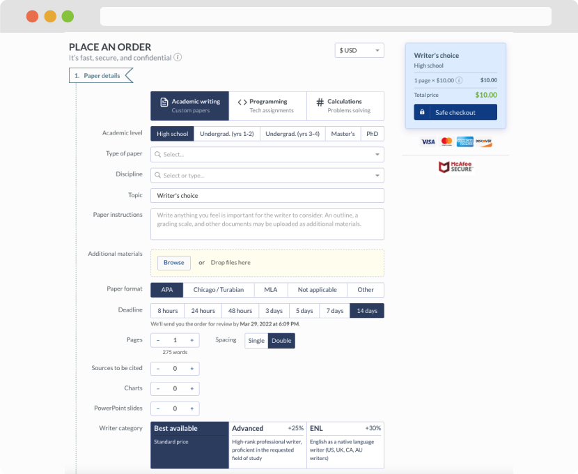
First, you will need to complete an order form. It's not difficult but, in case there is anything you find not to be clear, you may always call us so that we can guide you through it. On the order form, you will need to include some basic information concerning your order: subject, topic, number of pages, etc. We also encourage our clients to upload any relevant information or sources that will help.
Complete the order form
Once we have all the information and instructions that we need, we select the most suitable writer for your assignment. While everything seems to be clear, the writer, who has complete knowledge of the subject, may need clarification from you. It is at that point that you would receive a call or email from us.
Writer’s assignment
As soon as the writer has finished, it will be delivered both to the website and to your email address so that you will not miss it. If your deadline is close at hand, we will place a call to you to make sure that you receive the paper on time.
Completing the order and download