The analysis investigates the relation of credit card charges with Income and house hold size of 50 consumers. Table 1 presents the descriptive statistics of the Income ($000s) and amount charged on the credit card ($) of the client.
Table 1: Descriptive statistics for Income ($000s) and Amount Charged ($)
|
Descriptive Statistics |
Income ($1000s) |
Amount Charged ($) |
|
Mean |
43.48 |
3963.86 |
|
Median |
42 |
4090 |
|
Mode |
54 |
3890 |
|
Standard Deviation |
15 |
934 |
|
Kurtosis |
-1.25 |
-0.74 |
|
Skewness |
0.10 |
-0.13 |
|
Range |
46 |
3814 |
|
Minimum |
21 |
1864 |
|
Maximum |
67 |
5678 |
|
Sum |
2174 |
198193 |
|
Count |
50 |
50 |
The average (standard deviation) income ($000s) of the consumers is $43.48 ($15). The analysis shows that the minimum and maximum income of the consumers is $21 and $67 respectively. Hence the range of income of the consumers is $46. The median income of the consumers is $42. Maximum number of consumers of the organzation has an income of $54 (000s).
The average (standard deviation) of the amount charged by the client on credit cards is $3963.8 ($934). The analysis shows that the minimum and maximum amount charged for credit cards to the consumers is $1864 and $5678 respectively. Thus consumers are charged in the range of $3814 for credit card usage. $4090 is the median value charged on the credit card. Maximum number of consumers of the organization is charged $3890. (000s).
Table 2: Descriptive statistics for Household Size
|
House Hold Size |
Frequency |
|
1 |
5 |
|
2 |
15 |
|
3 |
8 |
|
4 |
9 |
|
5 |
5 |
|
6 |
5 |
|
7 |
3 |
Table 2 presents the house hold size of the consumers of the client. The analysis shows that most of the consumers (15) have a household size of 2. The maximum household size is 7, 3 consumers have the household size. The least household size is 1, there are 5 consumers which have the household size.
To investigate the relation between credit card charge by the client and income of the consumers a linear regression is carried out.
|
Table 3: Regression Statistics |
|
|
Multiple R |
0.6308 |
|
R Square |
0.3979 |
|
Adjusted R Square |
0.3853 |
|
Standard Error |
731.9025 |
|
Observations |
50 |
Table 4: Regression Coefficients
|
|
Coefficients |
Standard Error |
t Stat |
P-value |
|
Intercept |
2204.241 |
329.134 |
6.697 |
0.000 |
|
Income ($1000s) |
40.470 |
7.186 |
5.632 |
0.000 |
Table presents the regression coefficients for the relation between credit card charge and income of the consumers. The regression equation is represented as
Table 3 presents the regression statistics for the relation. The analysis shows that 39.79% of the variability in the amount charged on the credit card can be explained by the independent variable Income.
To investigate the relation between amounts charged on credit card by the client and the household size of the consumer a linear regression is carried out.
|
Table 5: Regression Statistics |
|
|
Multiple R |
0.7529 |
|
R Square |
0.5668 |
|
Adjusted R Square |
0.5578 |
|
Standard Error |
620.8163 |
|
Observations |
50 |
Table 6: Regression Coefficients
|
|
Coefficients |
Standard Error |
t Stat |
P-value |
|
Intercept |
2581.644 |
195.270 |
13.221 |
0.000 |
|
Household Size |
404.157 |
51.000 |
7.925 |
0.000 |
Table 6 presents the regression coefficients for the relation between credit card charge and household size of the consumers. The regression equation is represented as
Table 5 presents the regression statistics for the relation. The analysis shows that 56.68% of the variability in the amount charged on the credit card can be explained by the independent variable Household size.
The comparison of the R2 values shows that household size is a better predictor for amount charged on credit card.
To investigate the relation between income and household size of the consumers and amount charged on credit card by the client a multiple linear regression is carried done.
|
Table 7: Regression Statistics |
|
|
Multiple R |
0.9085 |
|
R Square |
0.8254 |
|
Adjusted R Square |
0.8179 |
|
Standard Error |
398.3249 |
|
Observations |
50 |
Table 8: Regression Coefficients
|
|
Coefficients |
Standard Error |
t Stat |
P-value |
|
Intercept |
1305.034 |
197.771 |
6.599 |
0.000 |
|
Income ($1000s) |
33.122 |
3.970 |
8.343 |
0.000 |
|
Household Size |
356.340 |
33.220 |
10.727 |
0.000 |
Table 8 presents the regression coefficients for the relation between amount charged on credit card and income and household size of the consumers. The regression equation is represented as
Table 7 presents the regression statistics for the relation. The analysis shows that 82.54% of the variability in the amount charged on the credit card can be explained through the independent variables Income ($000s) and Household size.
The regression equation for amount charged on credit card
Thus the amount that would be charged on a consumer whose household size is 3 as well as has an income of $40,000 is
Amount charged ($) = 1305.03 + 33.122*40 + 356.340*3
= 3698.93 ≈ 3699
Independent variables in a regression equation are helpful for predicting the variability in the dependent variable. The higher the value of R2 the better the model. Thus other independent variables which may help in developing a better model are
The variable Student ID is an identity variable. Thus the histogram for student ID cannot be created.
Table 9: Descriptive Statistics
|
|
Mean |
Standard Deviation |
Minimum |
Maximum |
|
Year Enrolled |
2013.04 |
0.81 |
2012 |
2014 |
|
HI001 FINAL EXAM |
31.72 |
6.75 |
0 |
45 |
|
HI001 ASSIGNMENT 01 |
17.21 |
1.99 |
8 |
22 |
|
HI001 ASSIGNMENT 02 |
15.46 |
2.31 |
8 |
21 |
|
HI002 FINAL EXAM |
26.50 |
5.91 |
0 |
40 |
|
HI002 ASSIGNMENT 01 |
17.82 |
3.44 |
4 |
22 |
|
HI002 ASSIGNMENT 02 |
12.42 |
1.99 |
4 |
16 |
|
HI003 FINAL EXAM |
25.99 |
8.27 |
4 |
43 |
|
HI003 ASSIGNMENT 01 |
18.19 |
3.91 |
10 |
30 |
|
HI003 ASSIGNMENT 02 |
13.54 |
1.76 |
8 |
20 |
Table 10: Correlation between variables
|
Sl. No. |
Correlation |
Karl-Pearson Correlation (r) |
Significance (p-value)* |
|
1 |
HI001 Final Exam and HI002 Final Exam |
0.049 |
0.630 |
|
2 |
HI001 Final Exam and HI003 Final Exam |
0.122 |
0.232 |
|
3 |
HI002 Final Exam and HI003 Final Exam |
0.116 |
0.257 |
|
4 |
HI001 Assignment 01 and HI001 Assignment 02 |
0.659 |
0.000 |
|
5 |
HI002 Assignment 01 and HI002 Assignment 02 |
0.549 |
0.000 |
|
6 |
HI003 Assignment 01 and HI003 Assignment 02 |
0.520 |
0.000 |
|
7 |
HI001 Final Exam and HI001 Assignment 01 |
0.093 |
0.364 |
|
8 |
HI002 Final Exam and HI002 Assignment 01 |
0.177 |
0.081 |
|
9 |
HI003 Final Exam and HI003 Assignment 01 |
0.197 |
0.052 |
|
10 |
HI003 Final Exam and HI003 Assignment 02 |
0.120 |
0.239 |
The Karl-pearsons correlation between HI001 Final Exam and HI002 Final Exam is r = 0.049. Thus the correlation can be said to be positive, very weak and linear. In addition the correlation is not statistically significant p-value = 0.630 > 0.05, level of significance.
The correlation between HI001 Final Exam and HI003 Final Exam is r = 0.122. Thus the correlation can be said to be positive, weak and linear. In addition the correlation is not statistically significant p-value = 0.232 > 0.05, level of significance.
The correlation between HI002 Final Exam and HI003 Final Exam is r = 0.116. Thus the correlation can be said to be positive, weak and linear. In addition the correlation is not statistically significant p-value = 0.257 > 0.05, level of significance.
The correlation between HI001 Assignment 01 and HI001 Assignment 02 is r = 0.659. Thus the correlation can be said to be positive, moderate and linear. In addition the correlation is statistically significant p-value < 0.001.
The correlation between HI002 Assignment 01 and HI002 Assignment 02 is r = 0.549. Thus the correlation can be said to be positive, moderate and linear. In addition the correlation is statistically significant p-value < 0.001.
The correlation between HI003 Assignment 01 and HI003 Assignment 02 is r = 0.520. Thus the correlation can be said to be positive, moderate and linear. In addition the correlation is statistically significant p-value < 0.001.
The correlation between HI001 Final Exam and HI001 Assignment 01 is r = 0.093. Thus the correlation can be said to be positive, very weak and linear. In addition the correlation is statistically not significant p-value =0.364 > 0.05, level of significance.
The correlation between HI002 Final Exam and HI002 Assignment 01 is r = 0.177. Thus the correlation can be said to be positive, weak and linear. In addition the correlation is statistically not significant p-value =0.081 > 0.05, level of significance.
The correlation between HI003 Final Exam and HI003 Assignment 01 is r = 0.197. Thus the correlation can be said to be positive, weak and linear. In addition the correlation is statistically not significant p-value =0.052 > 0.05, level of significance.
The correlation between HI003 Final Exam and HI003 Assignment 02 is r = 0.120. Thus the correlation can be said to be positive, weak and linear. In addition the correlation is statistically not significant p-value =0.239 > 0.05, level of significance.
Table 11: Depression Scores for individuals with reasonably good health
|
Depression Scores |
Florida |
New York |
North Carolina |
|
2 |
2 |
0 |
0 |
|
3 |
3 |
0 |
4 |
|
4 |
1 |
1 |
1 |
|
5 |
3 |
1 |
1 |
|
6 |
3 |
2 |
1 |
|
7 |
4 |
4 |
3 |
|
8 |
3 |
7 |
5 |
|
9 |
1 |
1 |
1 |
|
10 |
0 |
1 |
1 |
|
11 |
0 |
1 |
2 |
|
12 |
0 |
1 |
1 |
|
13 |
0 |
1 |
0 |
From the state of Florida individuals with reasonable good health had a depression score from 2 to 9. From the state of New York individuals with reasonable good health had a depression score from 4 to 13. From the state of North Carolina individuals with reasonable good health had a depression score from 3 to 12.
Table 12: Depression Scores for individuals with chronic health condition
|
Depression Scores |
Florida |
New York |
North Carolina |
|
8 |
0 |
0 |
1 |
|
9 |
1 |
2 |
0 |
|
10 |
1 |
0 |
1 |
|
11 |
1 |
2 |
2 |
|
12 |
3 |
1 |
3 |
|
13 |
3 |
1 |
2 |
|
14 |
1 |
4 |
3 |
|
15 |
2 |
2 |
2 |
|
16 |
2 |
1 |
1 |
|
17 |
4 |
2 |
2 |
|
18 |
0 |
1 |
2 |
|
19 |
0 |
1 |
1 |
|
20 |
1 |
1 |
0 |
|
21 |
1 |
0 |
0 |
|
22 |
0 |
0 |
0 |
|
23 |
0 |
1 |
0 |
|
24 |
0 |
1 |
0 |
Individuals with chronic health condition from Florida had a depression score from 9 to 21. Similarly individuals from New York had a depression score range of 9 to 24. Likewise individuals from North Carolina had a depression score in the range of 8 to 19.
Analysis of Variance is carried out to check for the relation between depression scores and geographical location
ANOVA 1 – Individuals with reasonably good health
Table 13: ANOVA for individuals with reasonably good health
|
Source of Variation |
SS |
df |
MS |
F |
P-value |
F crit |
|
Between Groups |
61.033 |
2 |
30.517 |
5.241 |
0.008 |
3.159 |
|
Within Groups |
331.900 |
57 |
5.823 |
|
|
|
|
Total |
392.933 |
59 |
|
|
|
|
The analysis of variance for individuals with reasonably good health shows that F(2,57) = 5.241. The p-value for the ANOVA = 0.008 < 0.05, level of significance. Thus, we reject the Null hypothesis.
Thus, it can be inferred that depressions scores of individuals with reasonably good health varies across geographical locations.
ANOVA 2 – Individuals with chronic health condition
Table 14: ANOVA for individuals with chronic health condition
|
Source of Variation |
SS |
df |
MS |
F |
P-value |
F crit |
|
Between Groups |
17.03 |
2 |
8.517 |
0.714 |
0.494 |
3.159 |
|
Within Groups |
679.70 |
57 |
11.925 |
|
|
|
|
Total |
696.73 |
59 |
|
|
|
|
The analysis of variance for individuals with chronic health conditions shows that F(2,57) = 0.714. The p-value for the ANOVA = 0.494 > 0.05, level of significance. Hence we do not reject the Null Hypothesis.
Thus, it can be inferred that depressions scores of individuals with chronic health conditions does not vary across geographical locations.
From the analysis of variance of depressions scores of individuals with good health and chronic health conditions it can be inferred:
Essay Writing Service Features
Our Experience
No matter how complex your assignment is, we can find the right professional for your specific task. Contact Essay is an essay writing company that hires only the smartest minds to help you with your projects. Our expertise allows us to provide students with high-quality academic writing, editing & proofreading services.
Free Features
Free revision policy
$10Free bibliography & reference
$8Free title page
$8Free formatting
$8How Our Essay Writing Service Works

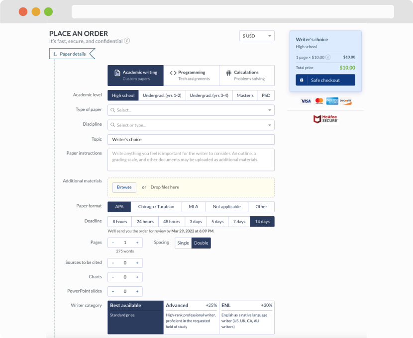
First, you will need to complete an order form. It's not difficult but, in case there is anything you find not to be clear, you may always call us so that we can guide you through it. On the order form, you will need to include some basic information concerning your order: subject, topic, number of pages, etc. We also encourage our clients to upload any relevant information or sources that will help.
Complete the order form
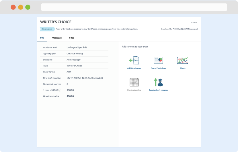
Once we have all the information and instructions that we need, we select the most suitable writer for your assignment. While everything seems to be clear, the writer, who has complete knowledge of the subject, may need clarification from you. It is at that point that you would receive a call or email from us.
Writer’s assignment
As soon as the writer has finished, it will be delivered both to the website and to your email address so that you will not miss it. If your deadline is close at hand, we will place a call to you to make sure that you receive the paper on time.
Completing the order and download