Define the Business Statistics for Nonparametric Models .
The level of measurement of the variable “Size” is nominal. This variable is measured in nominal scale as the values of the variable is differentiated based on the various sizes of the “compact”, “midsize” and “large” (Pedhazur and Schmelkin, 2013). The level of measurement of “displacement” is “ratio scale” as the values of the variable are measured in numbers. The level of measurement of “cylinders” is “ratio scale”. This is because the values of the variable give the magnitude of the “cylinders” of different sizes.
The level of measurement of “drive” is “ordinal”. This is because the variable is ordered according to their “wheels”. The variable is classified according to “all wheel”, “front wheel” and “rear wheel” which denotes the order of the variable. The level of measurement of the variable “fuel type” is ordinal (Gries, 2014). This is because the values of this variable are classified according to the “premium fuel” or “regular fuel”.
The variable “city MPG” has the level of measurement as “ratio scale”. This is because the values of the variable have a particular magnitude that gives the fuel efficiency rating for the city driving in terms of miles per gallon. The level of measurement of the variable “Hwy MPG” is ratio scale. This is because the there is a particular value for the samples of this variable which gives the measure of fuel efficiency rating for highway driving in terms of miles per gallon.
Refer to the excel file in the excel sheet “Data MG14”.
The histogram of cylinders is given below:
Figure 1: Histogram of the variable “cylinders”
(Source: Created by author)
The histogram of the variable “cylinders” show that the minimum value of the variable is 4 and the maximum value of the variable is 12. The frequency of maximum value of the variable “cylinder” is less. This shows that there are few cars that have maximum number of engines are 12. Most of the cars use 4, 6 or 8 engines. The histogram shows that the distribution of the variable is not normal, as the curve of the variable do not follow the curve of normal distribution.
Refer to the excel sheet “question f”.
The table of relative frequencies and percent frequencies for the frequency distribution of the variable “cylinders” is given below:
|
values |
relative frequency |
|
4 |
= (48 / 100) = 0.48 |
|
5 |
= (4 / 100) = 0.04 |
|
6 |
= (27 / 100) = 0.27 |
|
8 |
= (18 / 100) = 0.18 |
|
12 |
= (3 / 100) = 0.03 |
Table 1: Table of relative frequency of the variable “cylinders”
(Source: created by author)
|
values |
percentage frequency |
|
4 |
= (48/100) * 100 = 48 |
|
5 |
= (4/ 100) * 100 = 4 |
|
6 |
= (27 / 100) * 100 = 27 |
|
8 |
= (18 / 100) * 100 = 18 |
|
12 |
= (3 / 100) * 100 = 3 |
Table 2: Table of percentage frequency of the variable “Cylinders”
(Source: Created by author)
Refer to the excel sheet “question h”.
The pivot table constructed in excel is given below:
|
Count of Cylinders |
Column Labels |
|||||
|
Row Labels |
4 |
5 |
6 |
8 |
12 |
Grand Total |
|
Compact |
24 |
4 |
6 |
3 |
1 |
38 |
|
Large |
3 |
4 |
12 |
1 |
20 |
|
|
Midsize |
21 |
17 |
3 |
1 |
42 |
|
|
Grand Total |
48 |
4 |
27 |
18 |
3 |
100 |
Table 3: Pivot table using “size” as row label, “cylinders” as column label and “count of cylinders” as the values of the pivot table
(Source: created by author)
The probabilities are calculated using the pivot table created in the variable “cylinders”:
Total number of “cylinders” is 100. Number of cars that have 4 cylinders is 48.
The probability of selecting 4 cylinders at random is given by (48 / 100) = 0.48.
It was seen that the total number of cars is 100. Number of cars whose size is “compact”; i.e. small size is 38. The probability of randomly selecting a car, which has small size is given by (38 / 100) = 0.38.
The total number of cars chosen as samples is 100. The number of cars, which are small, is 38 and the number of cars which have 4 engines is 48. The number of small cars who have 4 engines is 24. The probability of selecting small cars which have 4 engines is given by 24 / 100 = 0.24.
The descriptive statistics calculated for the variable “City MPG” is given below:
|
City MPG |
|
|
Mean |
19.96 |
|
Standard Error |
0.468593425 |
|
Median |
19 |
|
Mode |
18 |
|
Standard Deviation |
4.68593425 |
|
Sample Variance |
21.9579798 |
|
Kurtosis |
3.204308984 |
|
Skewness |
1.073940138 |
|
Range |
30 |
|
Minimum |
11 |
|
Maximum |
41 |
|
Sum |
1996 |
|
Count |
100 |
|
Largest(1) |
41 |
|
Smallest(1) |
11 |
|
Confidence Level (95.0%) |
0.929790993 |
Table 4: descriptive statistics of “City MPG”
(Source: created by author)
The descriptive statistics calculated for the variable “Hwy MPG” is given below:
|
Hwy MPG |
|
|
Mean |
28.93 |
|
Standard Error |
0.520538765 |
|
Median |
29 |
|
Mode |
29 |
|
Standard Deviation |
5.205387652 |
|
Sample Variance |
27.09606061 |
|
Kurtosis |
0.059249286 |
|
Skewness |
0.163426126 |
|
Range |
24 |
|
Minimum |
18 |
|
Maximum |
42 |
|
Sum |
2893 |
|
Count |
100 |
|
Largest(1) |
42 |
|
Smallest(1) |
18 |
|
Confidence Level (95.0%) |
1.032861815 |
Table 5.: descriptive statistics of “Hwy MPG”
(Source: created by author)
On performing “descriptive statistics” on the variable “City MPG”, the mean value was found to be 19.96 while the value of standard deviation was found to be 4.68. It can be interpreted that the mean fuel efficiency rating for the city driving in miles per gallon is 19.96. The value of standard deviation is medium. It can be interpreted that the spread of fuel efficiency rating for city driving is deviated moderately from its mean value.
The descriptive statistics of the variable “Hwy MPG” shows that the mean value of the variable was 28.93 and the standard deviation of the variable was 5.20. It can be interpreted that the average rating of fuel efficiency for driving on highway in terms of miles per gallon is 28.93 (Weiss and Weiss, 2012). The rating shows that the efficiency of the fuel for driving on highways is high as the average value is high. The value of standard deviation shows that the efficiency of fuels deviates moderately from the mean with a value of 5.20. The deviation of the variable shows that the efficiency of fuels for driving on highway variers moderately across the cars.
The sample of “City MPG” and “Hwy MPG” drawn from its population is not given to follow normal distribution. Thus, it is assumed that the distribution of the population is t-distribution where the standard error of the population would be estimated from the sample drawn from the population and it would be used instead of standard deviation.
In order to calculate the margin of error for 95% confidence interval for the mean of the population of the variable “City MPG”, the standard error of the variable is found by (standard deviation / sqrt (n) = 4.68 / 10 = 0.468. The 95% critical value of this variable following t-distribution and having degree of freedom as 99 is given as 1.66. Therefore, the margin of error of “City MPG” at 95% confidence interval when the variable follows t-distribution is given by 1.66 * 0.468 = 0.7769.
In order to calculate the margin of error for 95% confidence interval for the mean of the population of the variable “Hwy MPG”, the standard error of the variable is found by (standard deviation / sqrt (n) = 5.20/ 10 = 0.520. The variable follows t-distribution and has the degrees of freedom as 99 (Bickel and Lehmann, 2012). The value of 95% confidence interval having 99 degrees of freedom is 1.66 (Kock, 2013). The margin of error for the variable “Hwy MPG” is 1.66 * 0.52 = 0.8632.
The 95% confidence interval for population mean of the variable “City MPG” is given by mean +(-) 1.66* standard error (Huang and Bentler, 2015). The lower 95% interval is given by 19.96 – (1.66 * 0.468) = 19.183 and the upper 95% interval is given by 19.96 + (1.66 * 0.468) = 20.736. The 95% confidence interval is given by 20.736 – 19.183 = 1.554. It can be interpreted that the 0.95 probability of containing the population mean is 1.554.
The 95% confidence interval for population mean of the variable “Hwy MPG” is given by mean +(-) 1.66* standard error. The lower 95% interval is given by 28.93 – (1.66*0.520) = 28.067 and the upper 95% interval is given by 28.93 + (1.66*0.520) = 29.793. The 95% confidence interval of “Hwy MPG” is given by 29.793 – 28.067 = 1.726. It can be interpreted that 0.95 probability of containing the population mean for this variable is 1.726.
0854 give the covariance between the variable “Displacement” and “City MPG”.
The correlation between the variable “Displacement” and “City MPG” is given by -0.72805.
0837 give the covariance between the variable “Displacement” and “Hwy MPG”.
The correlation between the variable “Displacement” and “Hwy MPG” is given by -0.81555.
The correlation coefficient between “Displacement” and “City MPG” was found to be -0.72805. It is seen that there is a strong negative relationship between the two variables. It can be interpreted that the change in one variable would have a strong effect on the other variable but in the opposite direction (Sang et al., 2016). This suggests that more is the value of “Displacement” less is the value of “City MPG”.
The correlation between “Displacement” and “Hwy MPG” was found to be -0.81555, which defines a strong negative association between these two variables. It can be interpreted that the change in one variable would strongly influence the change in another variable in the opposite direction (Shu and Nan, 2014). This suggests that higher the change in “Displacement”, lower is the value of “Hwy MPG”.
References
Bickel, P.J. and Lehmann, E.L., 2012. Descriptive statistics for nonparametric models IV. Spread. In Selected Works of EL Lehmann (pp. 519-526). Springer US.
Gries, S.T., 2014. Frequency tables: tests, effect sizes, and explorations.Glynn D, Robinson J. Polysemy and synonymy: corpus methods and applications in cognitive linguistics. Amsterdam: John Benjamins.
Huang, Y. and Bentler, P.M., 2015. Behavior of asymptotically distribution free test statistics in covariance versus correlation structure analysis.Structural Equation Modeling: A Multidisciplinary Journal, 22(4), pp.489-503.
Kock, N., 2013. Using WarpPLS in E-Collaboration Studies: Descriptive Statistics, Settings. Interdisciplinary Applications of Electronic Collaboration Approaches and Technologies, 62.
Pedhazur, E.J. and Schmelkin, L.P., 2013. Measurement, design, and analysis: An integrated approach. Psychology Press.
Sang, Y., Dang, X. and Sang, H., 2016. Symmetric Gini Covariance and Correlation. arXiv preprint arXiv:1605.02332.
Shu, H. and Nan, B., 2014. Large covariance/correlation matrix estimation for temporal data. arXiv preprint arXiv:1412.5059.
Weiss, N.A. and Weiss, C.A., 2012. Introductory statistics. London: Pearson Education.
Essay Writing Service Features
Our Experience
No matter how complex your assignment is, we can find the right professional for your specific task. Contact Essay is an essay writing company that hires only the smartest minds to help you with your projects. Our expertise allows us to provide students with high-quality academic writing, editing & proofreading services.
Free Features
Free revision policy
$10Free bibliography & reference
$8Free title page
$8Free formatting
$8How Our Essay Writing Service Works

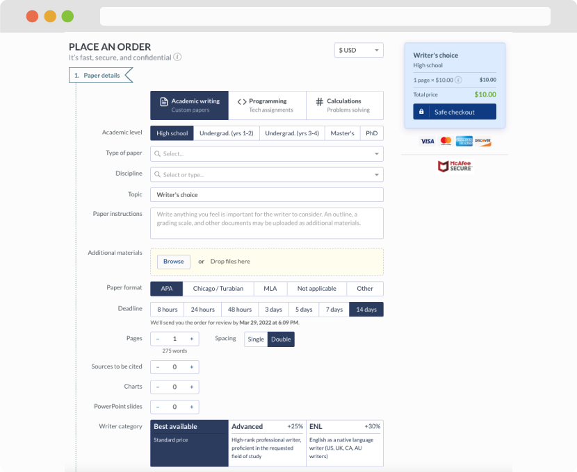
First, you will need to complete an order form. It's not difficult but, in case there is anything you find not to be clear, you may always call us so that we can guide you through it. On the order form, you will need to include some basic information concerning your order: subject, topic, number of pages, etc. We also encourage our clients to upload any relevant information or sources that will help.
Complete the order form
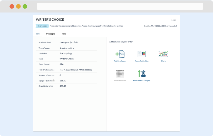
Once we have all the information and instructions that we need, we select the most suitable writer for your assignment. While everything seems to be clear, the writer, who has complete knowledge of the subject, may need clarification from you. It is at that point that you would receive a call or email from us.
Writer’s assignment
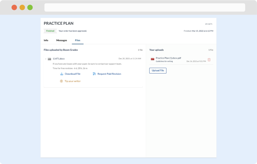
As soon as the writer has finished, it will be delivered both to the website and to your email address so that you will not miss it. If your deadline is close at hand, we will place a call to you to make sure that you receive the paper on time.
Completing the order and download