1. a. Frequency, relative frequency, percentage frequency with class limit points and mid points are evaluated and represented in the frequency table below (Black, 2009)
Table 1: Frequency Distribution table
| L.L | U.L | MID.POINT | CUM.FREQ | FREQ | REL.FREQ | CUM.REL.FREQ | PERCNT.REL.FREQ |
| $120.00 | $170.00 | $145.00 | 8 | 8 | 0.16 | 0.16 | 16% |
| $170.00 | $220.00 | $ 195.00 | 23 | 15 | 0.3 | 0.46 | 30% |
| $220.00 | $270.00 | $ 245.00 | 35 | 12 | 0.24 | 0.7 | 24% |
| $270.00 | $320.00 | $ 295.00 | 39 | 4 | 0.08 | 0.78 | 8% |
| $320.00 | $370.00 | $ 345.00 | 44 | 5 | 0.1 | 0.88 | 10% |
| $370.00 | $420.00 | $ 395.00 | 46 | 2 | 0.04 | 0.92 | 4% |
| $420.00 | $470.00 | $ 445.00 | 48 | 2 | 0.04 | 0.96 | 4% |
| $470.00 | $520.00 | $ 495.00 | 50 | 2 | 0.04 | 1 | 4% |
b. The above frequency table was used to draw the histogram and help of MS Excel has been taken for the purpose of drawing the diagram with percentage frequencies.
Figure 1: Histogram of the percent frequency distribution
c. The nature of the histogram was not normal, rather right skewed, which reflected that the data in the data set of Missy Walters were accumulated with high frequencies in the left tail. Median is used as a measure of central tendency when distribution is not normal in nature and hence it (median) was the best choice of measure of location. Mean can be used for any data set without outliers, but median is considered as a better choice as measure and was the appropriate selection as measure of location for this scenario (Montgomery, Runger & Hubele, 2009).
2.a. The regression equation was
The predictive model between demand and unit sale price was obtained from the above ANOVA and regression table. Due to increase in one unit price, it was noticed that demand abridged by 2.14 units, in the regression model. The adverse relation of demand and unit price was earlier explained by Economic theories.
b. Coefficient of determination was known to be
and was calculated accordingly. The completed ANOVA table was used, where SSE = 3132.66, SST = 8181.48,
It was inferred that unit price was an independent variable and was able to explain 62.0% variance of the dependent variable (demand).
c. The evaluation of the correlation coefficient was obvious and calculated as
it is to be noted that the negative sign was used, as the correlation coefficient and regression coefficient were considered of same sign .The correlation coefficient defined that there was statistically significant correlation between unit price and demand. The nature of the association was highly negative where unit price was a significant factor in measuring demand of an article.
3. a. Calculations were done to fill up the blank spaces in the ANOVA table using MS Excel as provided underneath.
Table 2: ANOVA Table for three treatments
| Source of variation | Sum of squares | Degrees of freedom | Mean square | f | p |
| Between Treatments |
390.58 |
2 |
195.29 | 2.89 | 0.00 |
| Within Treatments (Error) | 158.4 | 21 | 7.54 | ||
| Total | 548.98 |
23 |
202.83 |
The given values of SSE, SSB and SST were used for further calculations where degrees of freedom total was 11. For existence of three treatments m = 3, and for 24 observations n = 24. Therefore the total degree of freedom was n-1 = 23. Therefore the values were, SSE = 158.4, SSB = 390.58, SST = 548.98. Consequently calculated values were, MSB = SSB/ (m-1) =390.58/ 2 =195.29, MSE = SSE/ (n-m) = 158.4/ 21 =7.54, F = MSB / MSE = 195.29/ 7.54 = 25.89. The conforming significance level was less than 0.05 and it was observed that the outcome was significant at level of significance. The F value was 25.89 which at was in the critical region. Consequently the null hypothesis considering the three treatments to be equally effective was rejected (Heiberger & Neuwirth, 2009).
4. The ANOVA and Regression tables were completed using MS Excel as follows.
Table 3: ANOVA and Regression Data
ANOVA
| Df | SS | MS | f | p | |
| Regression | 2 | 40.7 | 20.35 | 80.1181102 | 0.000593 |
| Residual | 4 | 1.016 | 0.254 | ||
| Total | 6 | 41.716 | 20.604 |
Regression Table
| Coefficients | Standard Error | t | p | |
| Intercept | 0.8051 | 0.0698 | 11.54 | 0.00 |
| X1 | 0.4977 | 0.4617 | 1.08 | 0.33 |
| X2 | 0.4733 | 0.0387 | 12.23 | 0.00 |
The calculations used to complete the incomplete tables have been given below:
Total observations was, N = 7, consequently total degree of freedom was, N – 1 = 6. Existence of two independent variables indicated degrees of freedom for regression as 2, for residual DF was 4 (6 – 2 = 4). Currently, SSB = 40.7 and SSE = 1.016, so SST = (40.7 + 1.016) = 41.716. MSB = SSB /2 = 20.35, MSE = SSE/ 4 = 0.254. MST = MSB + MSE. The calculation of F value was done as the ratio between MSB and MSE. Significant value was evaluated using the F-distribution function (Albright, Winston & Zappe, 2010).
Standard error of intercept in regression analysis was found as
values were calculated as the proportion of coefficients and standard errors. The p-values were found using the t-distribution function.
a. Using the completed regression table, the estimated regression model was evaluated as
b. The null hypothesis: H0: There was no significant relation between mobiles sold and the independent factors, price and advertising spots.
c. The alternate hypothesis: HA: There was significant relation between mobiles sold and the independent factors, price and advertising spots.
Using the Regression table t-values for and variables were 1.08 (with p-value = 0.33) and 12.23 (with p-value < 0.05), it was apparent that variable X1 did not have significant correlation with number of phones sold per day (Y). Therefore, the estimated regression model was not statistically significant (Draper & Smith, 2014).
d. For the validity of association of the two regression coefficients, hypotheses were tested.
For the coefficient β1, the null hypothesis was: H0: β1 = 0 and alternate hypothesis was: HA: β1≠0.
The result was estimated using t-test where the statistic was evaluated as
(with p-value =0.33). Therefore the null hypothesis could not be rejected at level of significance. The first coefficient of price was not significantly different from zero (Cameron & Trivedi, 2013).
For the coefficient β2, let the null hypothesis was: H0: β2 = 0 and alternate hypothesis: HA: β2≠0.
The result was estimated using t-test where statistic was evaluated as
(with p-value < 0.05). Therefore the null hypothesis was rejected at level of significance. The coefficient was significantly different from zero.
e. The slope or intercept of the regression model was 0.8051 and the statement was that the coefficient had positive sign. Therefore it was inferred that mobiles sold per day had a significant sales figure when the independent influences were kept at zero.
Essay Writing Service Features
Our Experience
No matter how complex your assignment is, we can find the right professional for your specific task. Contact Essay is an essay writing company that hires only the smartest minds to help you with your projects. Our expertise allows us to provide students with high-quality academic writing, editing & proofreading services.
Free Features
Free revision policy
$10Free bibliography & reference
$8Free title page
$8Free formatting
$8How Our Essay Writing Service Works

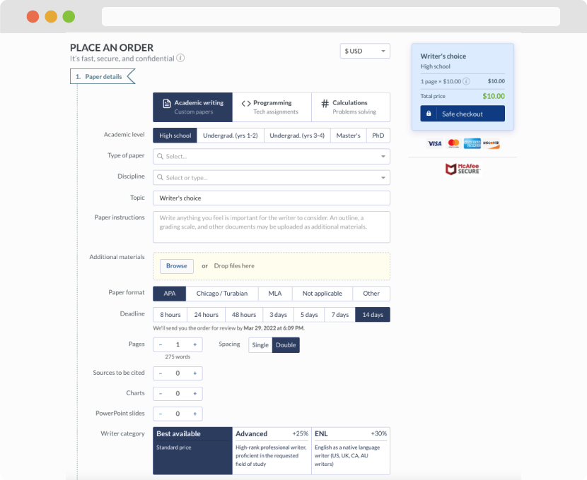
First, you will need to complete an order form. It's not difficult but, in case there is anything you find not to be clear, you may always call us so that we can guide you through it. On the order form, you will need to include some basic information concerning your order: subject, topic, number of pages, etc. We also encourage our clients to upload any relevant information or sources that will help.
Complete the order form
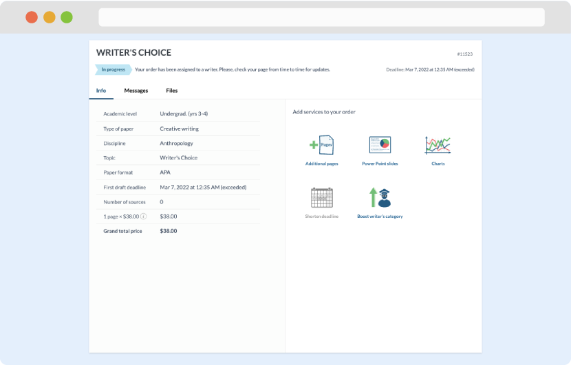
Once we have all the information and instructions that we need, we select the most suitable writer for your assignment. While everything seems to be clear, the writer, who has complete knowledge of the subject, may need clarification from you. It is at that point that you would receive a call or email from us.
Writer’s assignment
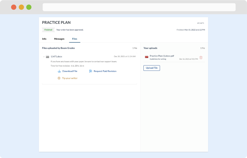
As soon as the writer has finished, it will be delivered both to the website and to your email address so that you will not miss it. If your deadline is close at hand, we will place a call to you to make sure that you receive the paper on time.
Completing the order and download