Part 1 – Preliminary Analysis
The report addresses the annual spending on food by consumers in the United States. The key research objectives are to determine whether the average annual expenditure on food for a household in Midwestern region of the United States is greater than $8,000 USD or not. Furthermore it looks to address whether the annual average household spending on food in a typical household from a metro area differs from one which is from those which are outside metro area. Also it investigates whether any difference exists in terms of annual expenditure on food, the household income per year and the non-mortgage housing debts between the four regions of the United States.
The data analysis is based on a sample of size 200. The dataset consists of observations on 200 households across the United States. It had five attributes, namely Annual Household expenditure in USD, Annual Household income in USD, Annual non-Mortgage debt, which are all quantitative continuous variables; the region where the household is from which is a categorical variable with 4 levels, namely, northeast(NE or 1), Midwest(MW or 2), south(S or 3) and west(W or 4); and finally the variable location which is also another categorical variable with the levels marking whether the household is from a Metro area(1) or from outside metro areas(2).
The analyses of the data to meet the requirements of the objectives that have been laid down has been done using statistical techniques of descriptive statistics, hypothesis testing and ANOVA analysis using Microsoft Excel.
Part 2 – Descriptive Statistics
The data was found to not have any outlier or any missing data..The average annual food spending was found to be 8966 USD with median value being 8932 USD. The standard deviation was found to be 3125.007 USD and the coefficient of variation was found to be 2.869. The minimum observed annual food expenditure of a household was found to be 2587 USD and the maximum observed annual food expenditure was found to be 17740 USD. 25% of the observed annual food spending of households in the sample or the first quartile value was found to be less than equal to 6933.75 USD whereas 75% of the observed annual food spending of households in the sample or the third quartile value was found to be less than 10950 USD. The mode of the values was computed from the grouped frequency distribution of the annual household expenditure on food and found to be equal to 9221.146 USD (Siegel, 2016) . The following table give the grouped frequency distribution of annual food spending. Figure 1 gives the histogram of the annual food spending of the households.
The average annual household income was found to be 55552 USD with median value being 54957.47 USD. The standard deviation was found to be 14661.3601 USD and the coefficient of variation was found to 3.7890. The minimum observed annual income of a household was found to be 21646.61 USD and the maximum observed annual food expenditure was found to be 96132.2 USD. 25% of the observed annual income of households in the sample or the first quartile value was found to be less than equal to 46162.965 USD whereas 75% of the observed annual income of households in the sample or the third quartile value was found to be less than 64933.543 USD. The mode of the values was computed from the grouped frequency distribution of the annual household income and found to be equal to 56400.71 USD (Siegel, 2016) . The following table give the grouped frequency distribution of annual income. Figure 2 gives the histogram of the annual income of the households.
|
Row Labels |
Count of Annual Household Income ($) |
|
21646.61-31646.61 |
8 |
|
31646.61-41646.61 |
36 |
|
41646.61-51646.61 |
33 |
|
51646.61-61646.61 |
62 |
|
61646.61-71646.61 |
30 |
|
71646.61-81646.61 |
24 |
|
81646.61-91646.61 |
6 |
|
91646.61-101646.61 |
1 |
|
Grand Total |
200 |
The average annual non-mortgage household debt was found to be 15604 USD with median value being 16100.24 USD. The standard deviation was found to be 8583.539 USD and the coefficient of variation was found to 1.8179. The minimum observed annual non-mortgage household debt was found to be 0 USD and the maximum observed annual food expenditure was found to be 36373.94 USD. 25% of the observed annual non-mortgage household debt in the sample or the first quartile value was found to be less than equal to 9191.929 USD whereas 75% of the annual non-mortgage household debt in the sample or the third quartile value was found to be less than 21259.127 USD. The mode of the values was computed from the grouped frequency distribution of annual non-mortgage household debt and found to be equal to 17333.33 USD (Siegel, 2016) . The following table give the grouped frequency distribution of annual income. Figure 3 gives the histogram of annual non-mortgage household debt.
Part 3 – Inferential Statistics
It is of interest to be seen whether the average food spending for the household in the Midwestern region of the US is greater than $8000 USD or not. The households from the Midwest regions are therefore considered and their average spending on food was seen to be $8659.689 USD. Then to test whether the food spending is greater than $8000 or not, a one sample t-test for means is employed (Zikmund et al., 2013). . The hypothesis to be tested could then be defined as follows:
H0A: Average annual household expense on food in Midwestern households equals $8000
H1A: Average annual household expense on food in Midwestern households is greater than $8000
The p-value was found to be 0.0323 and the null hypothesis (H0A) thus could not be at 1% level of significance (Ott & Longnecker, 2015).This means that not enough evidence was found to support the claim that the annual household expenditure on food is greater than $8000 among households in the Midwest.
Additionally, it is of interest to gauge whether there is any significant discrepancy in the annual expenditure for food between those households which are from metro areas and those which are from outside metro areas. The level of the test was taken to be α = 0.01. Then, to test for the difference in the expenditure amounts between the regions the data for the households in metro regions and those falling outside were grouped accordingly and the average spending was found to be $9435.933 for those in region 1, that is, metro regions and $8261.262 for those in region 2, that is, outside metro regions (Lowry, 2014). The conjectures to be contested could thus be defined as follows:
H0B: The average annual spending on food of households in metro regions equals that of those outside metro regions
H1B: The average annual spending on food of households in metro regions does not equal that of those outside metro regions
The p-value for the independent two sample t-test used to test for the conjectures was found to be 0.0071 which is less than 0.01 which is the level of significance. Therefore the null hypothesis (H0B) was rejected at 1% level of significance (Berenson et al., 2012).This means that there is enough evidence to suggest that the annual spending on food in the households in areas falling within metro regions differ significantly to those which fall outside of them.
Finally it is to be determined whether the four regions Midwest, Northeast, West and South differ in terms of annual household income, annual spending on food and annual non-mortgage debt or not. To test for the difference among the regions in terms of annual spending on food the hypotheses to be tested can be defined as follows:
H0C1 : There is no difference in the average food spending among the four regions
H1C1 : There is differences in the average food spending among the four regions.
The ANOVA test was used to test for the validity of the above conjecture (Myers et al, 2013). The F-statistic was found to be 3.48 and the critical value was found to be 3.909. The p-value was found to be 0.017. Thus there was not enough evidence to reject the null hypothesis (H0C1) at 1% level of significance. This means that no difference exists among annual food spending of the regions.
To test for the difference among the regions in terms of annual household income the hypotheses to be tested can be defined as follows:
H0C2 : There is no difference in the average annual household income among the four regions
H1C2 : There is differences in the average annual household income among the four regions
The ANOVA test was used to test for the validity of the above conjecture. The F-statistic was found to be 2.59 and the critical value was found to be 2.68. The p-value was found to be 0.05. Thus there was not enough evidence to reject the null hypothesis (H0C2) at 1% level of significance. This means that there does not exist difference between annual household income of the regions (Wasserman, 2013). .
To test for the difference among the regions in terms of non-mortgage debt the hypotheses to be tested can be defined as follows:
H0C3 : There is no difference in the average non-mortgage debt among the four regions
H1C3 : There is differences in the average non-mortgage debt among the four regions
The ANOVA test was used to test for the validity of the above conjecture. The F-statistic was found to be 5.71 and the critical value was found to be 2.65 (Lowry, 2014).The p-value was found to be 0.009. This implies that the null hypothesis (H0C3) is rejected at 1% level of significance. This means that there does exist difference between non-mortgage debt of the regions (Hair et al., 2015).
Part 4 – Conclusion and Recommendations
The data had no missing data or outliers. The subsequent analysis revealed that annual spending on food was not greater than $8000 USD. It could also be said that the annual food spending of households in metro regions are greater than households which lie outside the regions. Again it can be concluded that there is no general difference in annual household income among the four regions Midwest, Northeast, West and South. Additionally it could be asserted that there is no general difference in annual food spending among these four regions. However no significant discrepancies exist among the non-mortgage debts among these regions.
References:
Berenson, M., Levine, D., Szabat, K. A., & Krehbiel, T. C. (2012). Basic business statistics: Concepts and applications. Pearson higher education AU.
Hair Jr, J. F., Wolfinbarger, M., Money, A. H., Samouel, P., & Page, M. J. (2015). Essentials of business research methods. Routledge.
Lowry, R. (2014). Concepts and applications of inferential statistics.
Myers, J. L., Well, A. D., & Lorch Jr, R. F. (2013). Research design and statistical analysis. Routledge.
Ott, R. L., & Longnecker, M. T. (2015). An introduction to statistical methods and data analysis. Nelson Education.
Schroeder, L. D., Sjoquist, D. L., & Stephan, P. E. (2016). Understanding regression analysis: An introductory guide (Vol. 57). Sage Publications.
Siegel, A. (2016). Practical business statistics. Academic Press.
Triola, M. F. (2013). Elementary statistics using Excel. Pearson.
Wasserman, L. (2013). All of statistics: a concise course in statistical inference. Springer Science & Business Media.
Zikmund, W. G., Babin, B. J., Carr, J. C., & Griffin, M. (2013). Business research methods. Cengage Learning.
Essay Writing Service Features
Our Experience
No matter how complex your assignment is, we can find the right professional for your specific task. Contact Essay is an essay writing company that hires only the smartest minds to help you with your projects. Our expertise allows us to provide students with high-quality academic writing, editing & proofreading services.
Free Features
Free revision policy
$10Free bibliography & reference
$8Free title page
$8Free formatting
$8How Our Essay Writing Service Works

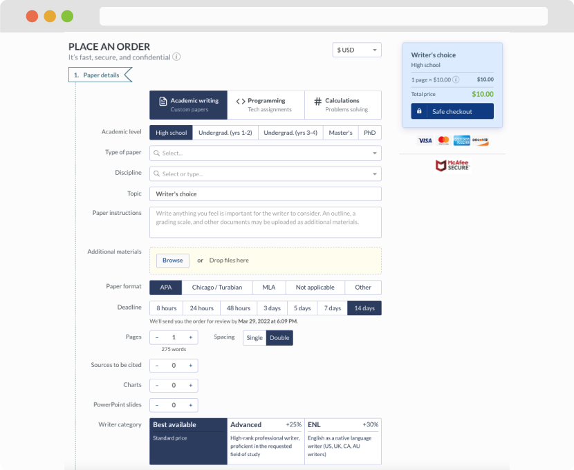
First, you will need to complete an order form. It's not difficult but, in case there is anything you find not to be clear, you may always call us so that we can guide you through it. On the order form, you will need to include some basic information concerning your order: subject, topic, number of pages, etc. We also encourage our clients to upload any relevant information or sources that will help.
Complete the order form
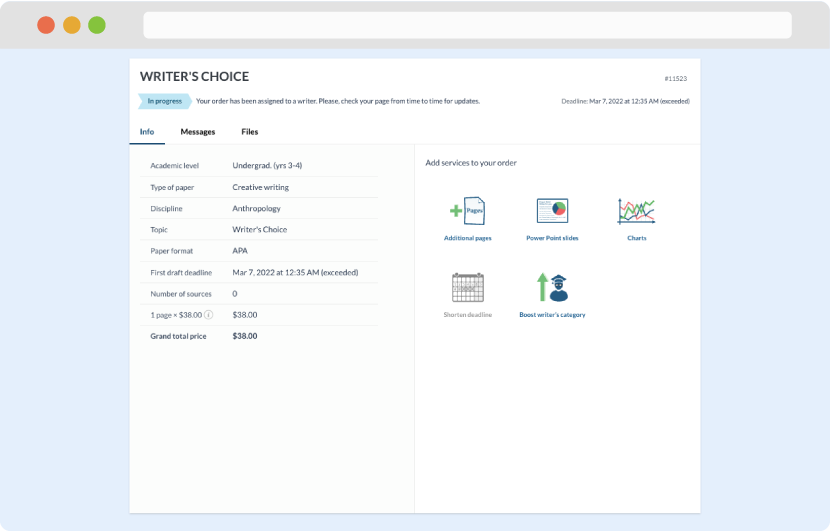
Once we have all the information and instructions that we need, we select the most suitable writer for your assignment. While everything seems to be clear, the writer, who has complete knowledge of the subject, may need clarification from you. It is at that point that you would receive a call or email from us.
Writer’s assignment
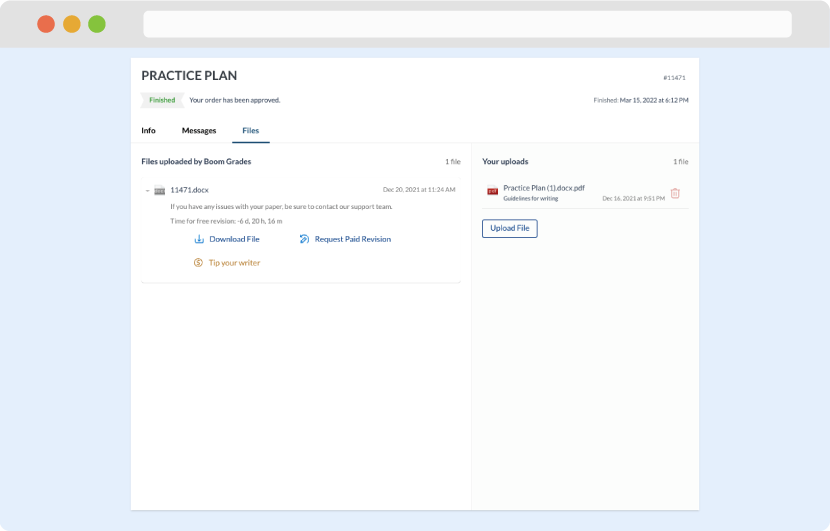
As soon as the writer has finished, it will be delivered both to the website and to your email address so that you will not miss it. If your deadline is close at hand, we will place a call to you to make sure that you receive the paper on time.
Completing the order and download