Security Market Line is representation in visual form of Capital Asset Pricing Model (CAPM). This line depicts the relationship between the expected return of an asset or security with its Beta coefficient (a measure of systematic risk of such security). In layman terms, it depicts risk return relationship for a given beta or return risk relationship for a given expected return.
The formula for the Security Market Line in terms of CAPM equation has been depicted here-in-below:
Expected Return= Risk Free Rate of Return + Beta coefficient of Security ( Risk Premium) ;
Whereby formula for Risk Premium is Market Rate of Return – Risk Free rate of Return.
Capital Market Line (CML) is a graph that depicts relationship between expected return of a portfolio encompassing all possible proportions between the market portfolio and risk free asset. Also the expected return represents the return of market as a whole. The formula for generation of expected return of a portfolio is shown here-in-below:
Expected Return of a Portfolio= Proportion of Market Portfolio * Expected Return of Market Portfolio* (1- Proportion of Market Portfolio)* Risk Free Rate.
Further under CML, the return of a non-leveraged portfolio can be less or equal to market portfolio. However, the return of a leveraged portfolio can exceed the return of market portfolio.
Comparison Analysis of Difference
Let us assume that the risk free rate of return is 5%;
Return on Australian ASX 200 is 10%
Then Risk premium is 5%.
Further let the total risk of portfolio be 8% and non-diversifiable risk of security be 0.25.
Further market Standard deviation is 8%
Then According to SML rate of return is =5% +0.25*5%=6.25%.
Then According to CML rate of return is =5% +[(5%/8%]*10%=11.25%
Let us first understand the meaning of minimum variance portfolio which is a well-diversified portfolio that is composed of assets that are risky on an individual basis but when they from a part of portfolio their overall risk is reduced with a given level of anticipated return. It is one of the significant portfolio optimising tool which maximises return and minimizes risk which is generally the goal of rationale investor.
For building a minimum variance portfolio, an investor needs to make a combination of difference securities with different level of risk generally low level or securities with low correlation with each other. Further, with low correlation is the most common method of building minimum variance portfolio.
In short, minimum variance portfolio is a diversified portfolio with securities having a low or negative correlation for a given level of return with an intention to reduce risk.
Suppose an individual has portfolio consisting of 100% shares and return of 15% and risk of 18% while other individual has return of 7% and risk of 10% by investing in bonds and a third individual has return of 11% by investing in international market of 13%.. The Minimum variance portfolio can be achieved by creating an optimum combination of all three portfolio in such a manner that the return on such investment shall exceed 11% and the risk of such investment shall be lower than 13%. Let us assume that combination is 30% of shares, 30% of Bond and 40% of international market. This represents the minimum variance portfolio.
Let us take another example under which there are only 5 stocks in the investment horizon and the weight, rate of return over 9 years have been tabulated here-in-below:
|
Weights |
15% |
20% |
12% |
36% |
17% |
|
Year |
Stock A |
Stock B |
Stock C |
Stock D |
Stock E |
|
1 |
21.46% |
12.53% |
20.32% |
7.48% |
15.65% |
|
2 |
-6.54% |
-1.49% |
4.95% |
4.16% |
1.21% |
|
3 |
6.05% |
0.02% |
0.72% |
9.97% |
1.37% |
|
4 |
-3.78% |
-3.41% |
10.82% |
-1.47% |
2.92% |
|
5 |
-0.16% |
-6.22% |
1.93% |
1.17% |
-3.49% |
|
6 |
-3.33% |
1.08% |
-3.93% |
-5.06% |
-9.49% |
|
7 |
-9.95% |
-11.81% |
-8.48% |
-0.37% |
7.80% |
|
8 |
-5.34% |
-11.45% |
-18.64% |
-19.69% |
-10.37% |
|
9 |
16.75% |
15.65% |
26.64% |
13.19% |
13.18% |
|
Average |
1.68% |
-0.81% |
3.81% |
1.04% |
2.09% |
|
Standard Deviation |
10.88% |
9.51% |
14.02% |
9.71% |
9.10% |
|
Annual Return |
22.19% |
-9.25% |
56.72% |
13.27% |
28.11% |
Further annual return has been computed by taking the formula (1+ average return)*time-1
Also the correlation and covariance between the stocks presented here-in-below:
|
Correlation |
A |
B |
C |
D |
E |
|
A |
1 |
0.71 |
0.7 |
0.5 |
0.67 |
|
B |
0.71 |
1 |
0.69 |
0.56 |
0.55 |
|
C |
0.7 |
0.69 |
1 |
0.62 |
0.63 |
|
D |
0.5 |
0.56 |
0.62 |
1 |
0.6 |
|
E |
0.67 |
0.55 |
0.63 |
0.6 |
1 |
|
Covariance |
A |
B |
C |
D |
E |
|
A |
0.0105 |
0.0028 |
0.0039 |
0.002 |
0.0025 |
|
B |
0.0028 |
0.008 |
0.0034 |
0.002 |
0.0018 |
|
C |
0.0039 |
0.0034 |
0.0175 |
0.003 |
0.0028 |
|
D |
0.002 |
0.002 |
0.003 |
0.0084 |
0.002 |
|
E |
0.0025 |
0.0018 |
0.0028 |
0.002 |
0.0074 |
Thus optimised portfolio is presented here-in-below
|
Optimised Porfolio |
|||||
|
A |
B |
C |
D |
E |
|
|
Weight |
15% |
20% |
12% |
36% |
17% |
|
15% |
0.0002 |
0.0001 |
0.0001 |
0.0003 |
0.0001 |
|
20% |
0.0001 |
0.0003 |
0.0001 |
0.0001 |
0.0001 |
|
12% |
0.0001 |
0.0001 |
0.0003 |
0.0001 |
0.0001 |
|
36% |
0.0000 |
0.0001 |
0.0001 |
0.0011 |
0.0001 |
|
17% |
0.0001 |
0.0001 |
0.0001 |
0.0001 |
0.0002 |
|
Total |
0.0005 |
0.0007 |
0.0005 |
0.0016 |
0.0006 |
|
Variance |
0.40% |
||||
|
Standard Deviation |
6.29% |
||||
|
Return |
17.84% |
On the basis of above, one may see that return has increased and risk has minimised.
The graph of minimum variance portfolio is presented here- in- below;
The importance of Minimum Variance Portfolio has been detailed here-in-below:
Capital Asset Pricing Model is a financial model that depicts relationship between systematic risk i.e. Beta and expected rate of return. It is an additive model. The formula for computation of expected return has been depicted here-in-below:
RT
The Computation under CAPM is based on two notions:
The other models that are common for computation of expected return include dividend discount Model, weighted Average Cost of Capital and others.
The first and foremost significance and relevance of CAPM is on account of its ease of computation. The formula for computation is simple and represents only two portions time value of money represented by Risk free rate and risk represented by Beta and market premium. Further, the method can be easily stress tested to compute a wide array of values of outcome to provide confidence and range to investor of possible rate of return.
The assumption of investor holding a diversified portfolio is in alignment with market portfolio and minimum variance portfolio and thus useful. Further, due to diversification only systematic risk i.e. Beta shall be taken into consideration.
Further, CAPM takes into account Systematic which is not considered under other models like Dividend Discount Model. This is a significant part of investment analysis and can never be overlooked while making an investment in security.
In addition, business and financial risk variability compatibility is present under CAPM which is missed out under Weighted Average Cost of Capital method. Thus if the current mix of debt equity is not in alignment with the proposed project, then even CAPM can be used for computation of return.
The model of CAPM is theoretically derived and has been subject to many back testing. It has been established based on frequent empirical research and testing.
The model further considers a wider picture taking market as a whole rather than being confined to the company as done under other models. The model considers market rate of return which is missing in other models and thus predict a more realistic and accurate model. Further, research and studies have predicted a very high rate of success of CAPM compared to other models for computation of expected return.
Further, one more advantage of using CAPM is that it provides rate of discount for appraising a project which is absent under WACC method. Thus, it is more convenient compared to WACC.
In addition, CAPM model can be used for computation of expected return even if the company is paying dividend or not which is absent under dividend discount model which is dependent on dividend for computation of return.
Thus, on the basis of above it can be understood that CAPM simplify and ease the work of financial investor and decision makers. The decision makers can use this model in conjunction with traditional techniques and a healthy judgement to predict pragmatic and useful estimates of expected return.
Essay Writing Service Features
Our Experience
No matter how complex your assignment is, we can find the right professional for your specific task. Contact Essay is an essay writing company that hires only the smartest minds to help you with your projects. Our expertise allows us to provide students with high-quality academic writing, editing & proofreading services.
Free Features
Free revision policy
$10Free bibliography & reference
$8Free title page
$8Free formatting
$8How Our Essay Writing Service Works

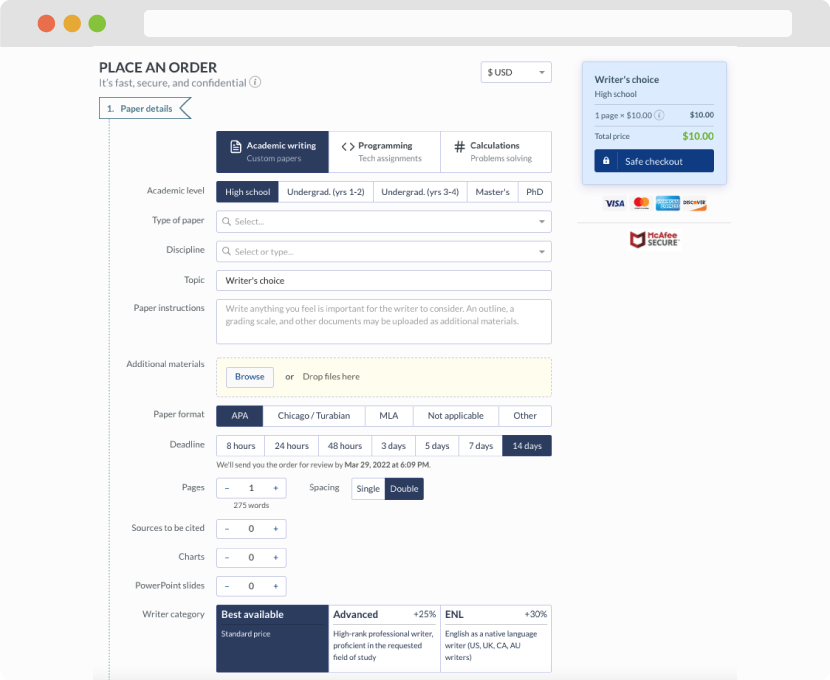
First, you will need to complete an order form. It's not difficult but, in case there is anything you find not to be clear, you may always call us so that we can guide you through it. On the order form, you will need to include some basic information concerning your order: subject, topic, number of pages, etc. We also encourage our clients to upload any relevant information or sources that will help.
Complete the order form
Once we have all the information and instructions that we need, we select the most suitable writer for your assignment. While everything seems to be clear, the writer, who has complete knowledge of the subject, may need clarification from you. It is at that point that you would receive a call or email from us.
Writer’s assignment
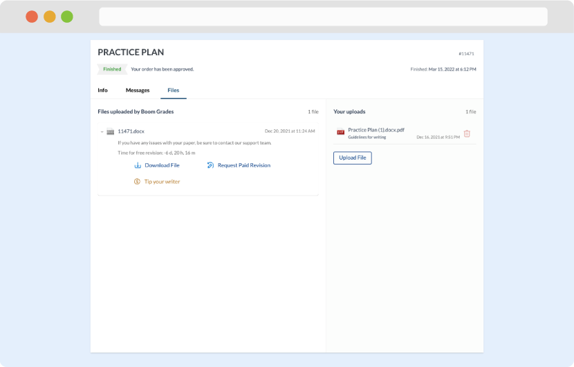
As soon as the writer has finished, it will be delivered both to the website and to your email address so that you will not miss it. If your deadline is close at hand, we will place a call to you to make sure that you receive the paper on time.
Completing the order and download